A Step-by-step Implementation of a Trading Strategy in Python using ARIMA + GARCH models

The post “A Step-by-step Implementation of a Trading Strategy in Python using ARIMA + GARCH models” first appeared on Medium, and it has been kindly contributed to the IBKR Quant Blog by the author.

Excerpt

Make use of a completely functional ARIMA+GARCH python implementation and test it over different markets using a simple framework for visualization and comparisons.

Introduction

When it comes to financial Time Series (TS) modelling, autoregressive models (models that makes use of previous values to forecast the future) such as ARMA, ARIMA or GARCH and its various variants are usually the preferred ones to explain the foundations of TS modelling. However, practical application of these techniques in real trading strategies and it’s comparison to naïve strategies (like Buy and Hold) are not that common. Moreover, it’s not easy to find a ready to use implementation that could be easily replicated for other markets, assets, etc. Some of the codes that I had run into have failures or are just incomplete and missing something. To make things even more difficult, the good implementations are written in R and the packages to fit the models in python and in R have some important differences that we will be exploring throughout this article.

In this context, the idea of this post it not to explain the concepts of these methods or the fundamental concepts of TS modelling. For that, you can refer to these free (and good) content available on the web:

• Online book — Forecasts: Principles and Practice
• QuantStart
• Auquan
• Machine Learning Mastery
• Analytics Vidhya

The Baseline

In order to guarantee that we have a good (reliable and robust) python implementation of a ARIMA+GARCH trading strategy, I will rely on the tutorial provided by QuantStart (here) that employed a R implementation on the S&P 500 index from 1950 to 2015 with consistent results that are significantly higher than a Buy and Hold strategy. To have all the parameters under control, instead of using their output signal as a baseline, I will replicate the code, re-run the tests and extend the testing period to December of 2020.

I had to make some small adjustments and I’ve added some exception handling to the original R script to successfully execute it. I don’t know if it is something related to package versioning, but considering that the R code is not our final objective I didn’t spend much time trying to understand the reasons and just put the code to run. Here is my version of the script:

install.packages("quantmod")
install.packages("lattice")
install.packages("timeSeries")
install.packages("rugarch")

library(quantmod)
library(lattice)
library(timeSeries)
library(rugarch)

# Added
library(xts)

getSymbols("^GSPC", from="1950-01-01")
spReturns = diff(log(Cl(GSPC)))
spReturns[as.character(head(index(Cl(GSPC)),1))] = 0

windowLength = 500
foreLength = length(spReturns) - windowLength
forecasts <- vector(mode="character", length=foreLength)

ini = 0
for (d in ini:foreLength) {
  # Obtain the S&P500 rolling window for this day
  spReturnsOffset = spReturns[(1+d):(windowLength+d)]
  
  # Fit the ARIMA model
  final.aic <- Inf
  final.order <- c(0,0,0)
  for (p in 0:5) for (q in 0:5) {
    if ( p == 0 && q == 0) {
      next
    }
    
    arimaFit = tryCatch( arima(spReturnsOffset, order=c(p, 0, q)),
                         error=function( err ) {
                           message(err)
                           return(FALSE)
                         },
                         warning=function( err ) {
                           # message(err)
                           return(FALSE)
                         } )
    
    if( !is.logical( arimaFit ) ) {
      current.aic <- AIC(arimaFit)
      if (current.aic < final.aic) {
        final.aic <- current.aic
        final.order <- c(p, 0, q)
        # final.arima <- arima(spReturnsOffset, order=final.order)
        final.arima <- arimaFit
      }
    } else {
      next
    }
  }
  
  # test for the case we have not achieved a solution  
  if (final.order[1]==0 && final.order[3]==0) {
    final.order[1] = 1
    final.order[3] = 1
  }
  
  
  # Specify and fit the GARCH model
  spec = ugarchspec(
    variance.model=list(garchOrder=c(1,1)),
    mean.model=list(armaOrder=c(final.order[1], final.order[3]), include.mean=T),
    distribution.model="sged"
  )
  fit = tryCatch(
    ugarchfit(
      spec, spReturnsOffset, solver = 'hybrid'
    ), error=function(e) e, warning=function(w) w
  )
  
  # If the GARCH model does not converge, set the direction to "long" else
  # choose the correct forecast direction based on the returns prediction
  # Output the results to the screen and the forecasts vector
  if(is(fit, "warning")) {
    forecasts[d+1] = paste(index(spReturnsOffset[windowLength]), 1, sep=",")
    print(paste(index(spReturnsOffset[windowLength]), 1, sep=","))
  } else {
    fore = ugarchforecast(fit, n.ahead=1)
    ind = fore@forecast$seriesFor
    forecasts[d+1] = paste(colnames(ind), ifelse(ind[1] < 0, -1, 1), sep=",")
    print(paste(colnames(ind), ifelse(ind[1] < 0, -1, 1), sep=",")) 
  }
}
write.csv(forecasts, file="/forecasts_test.csv", row.names=FALSE)

ARIMA.r hosted with ❤ by GitHub

If the script stops for any reason (it happened to me without any previous warning) just adjust the ini variable at the beginning of the loop to the last d calculated and re-run it, you will not lose any work. Two days and some restarts later, my 17366 forecasts days were finally created. Just as the original author did, I will leave the file here (sp500_forecasts_new.csv) if you want to download it directly.

Now that we have our predictions, it is time to test it in a simple strategy. Our strategy will simply long the position if the prediction is 1 (up) and short if the prediction is -1 (down). No considerations of slippage, transaction costs, etc. will be taken into account and we will consider that we enter the position at the opening price and exit the position at the closing price of the day.

Baseline Results

At this point, different from the original post, we will implement the strategy results in python. If you have downloaded the sp500_forecasts_new.csv from my GitHub will have the adjusted version. Refer to the QuantStart post for more details.

To download the original data from S&P500, we will use de yfinance package that can be easily installed using pip install yfinance.

• Step 1 — Opening the forecasts: First of all, we will open the forecasts CSV as a pandas DataFrame and set the Date as the index of the table (Note: the index has to be converted to DateTime type). That will make things easier when joining values along the index.
• Step 2 — Load the S&P500 values using yfinance and adjust the dates to match those of the forecasts.
• Step 3 — Join the columns

import pandas as pd
import numpy as np
import yfinance as yf

# Load the forecasts
forecasts = pd.read_csv('sp500_forecasts_new.csv', header=None).rename(columns={0: 'Date', 1: 'Signal'})
forecasts.set_index('Date', inplace=True)
forecasts.index = pd.to_datetime(forecasts.index)

# load the SP500 df
df = yf.Ticker('^GSPC').history(period='max')
df = df[(df.index > '1952-01-03') & (df.index < '2020-12-30')]

# save the strategy signal
df['Signal'] = forecasts['Signal']
df.head()

arima1.py hosted with ❤ by GitHub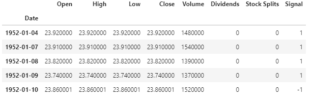

Once we have everything in one DataFrame, we will calculate the strategy return in a simple way. First we will create the Log Returns for the Close value of the index. The strategy Log Returns will be just the Log Returns multiplied by the Signal. If both has the same signal, our strategy return will be positive with the same value of the Log Return. If the signals are opposite, our strategy return will be negative. Of course, that it takes into account that we are shortening the position and can be adjusted if wanted. Another point to be considered is that we are not considering slippage or trading commissions and we are capturing all the variation of the day considering the closing of the previous day, and not the opening value. To make all these considerations, one could use a full featured backtesting framework like Backtrader.

To check the overall gains from the Buy and Hold and the strategy, we just have to accumulate the sum of the Log Returns.

For additional insight on the ARIMA+GARCH model tutorial visit https://cordmaur.carrd.co/#finance. For information about the course Introduction to Python for Scientists (available on YouTube) and other articles like this, visit cordmaur.carrd.co.