An Introduction to Probabilistic Deep Learning Explained in Simple Terms

Excerpt

Deep learning is nothing else than probability. There are two principles involved in it, one is the maximum likelihood and the other one is Bayes.  It is all about maximizing a likelihood function in order to find the probability distribution and parameters that best explain the data we are working with. Bayesian methods come into play where our network needs to say, “I am not sure”. It is at the crossing between deep learning architecture and Bayesian probability theory.

In general deep learning can be described as a machine learning technique based on artificial neural networks. To give you an idea of what an artificial neural network looks like see figure 1.

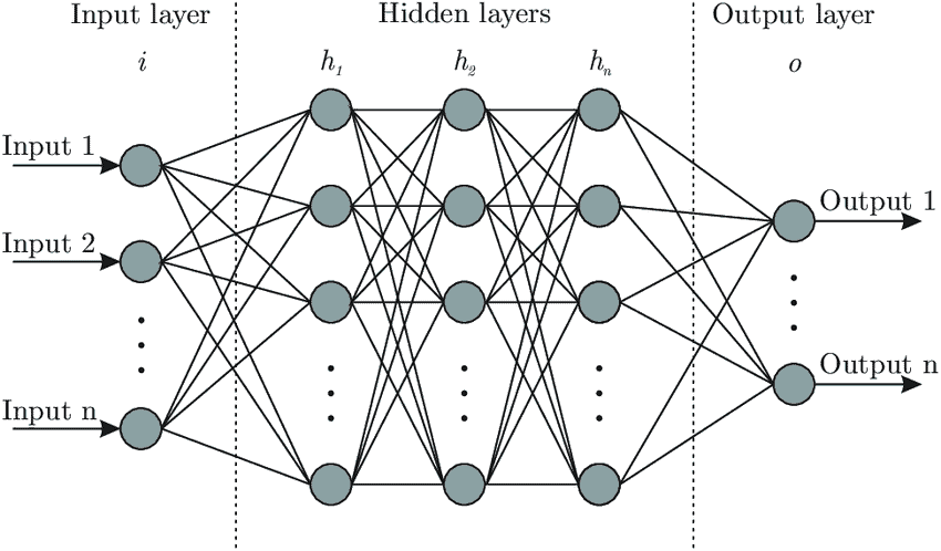
Figure1. Example artificial neural network with three hidden layers.

In figure 1 you can see an artificial NN with three hidden layers and several neurons on each layer. Each neuron is connected with each neuron in the next layer. The network simulates the way the human brain analyzes and processes information. While the human brain is quite complex, a neuron in an artificial NN is a simplification of its biological counterpart.

To get a better understanding imagine a neuron as a container for a number. The neurons in the input layer are holding the numbers. Such input data could be the historical volatility, and implied volatility of the S&P 500 Index. The neurons in the following layers get the weighted sum of the values from the connected neurons. The connections aren’t equally important, weights determine the influence of the incoming neuron’s value on the neuron’s value in the next layer. With the training data you tune the weights to optimally fit the data. Only after this step the model can be used for predictions.

Working with a deep learning system consists of two steps.

1. Choosing the architecture for your given problem
2. Tune the weights of the model

Classification

Classification involves predicting which class an item belongs to. Most classification models are parametric models, meaning the model has parameters that determine the course of the boundaries. The model can perform a classification after replacing the parameters by certain numbers. Tuning the weights is about how to find these numbers. The workflow can be summarized in three steps:

1. Extracting features from the raw data
2. Choosing a model
3. Fitting classification model to the raw data by tuning the parameter

By using validation data you evaluate the performance of the model. It is similar to a walk forward analysis where you use the data set not used during the optimization of your parameters.

We differentiate between probabilistic and non-probabilistic classification models.

Probabilistic classification

It refers to a scenario where the model predicts a probability distribution over the classes. As an example from the stock market, a probabilistic classifier would take financial news and then output a certain probability of the stock market going up or down. Both probabilities add up to one. You would pick the trade with the highest probability.

However, if you provide the classifier with an input not relevant to the security the classifier has no other choice than assigning probabilities to the classes. You hope that the classifier shows its uncertainty by assigning more or less equal probabilities to the other possible but wrong classes. This is often not the case in probabilistic neural network models. This problem can be tackled if we extend the probabilistic models by taking a Bayesian approach.

Bayesian probabilistic classification

Bayesian Classification is a naturally probabilistic method that performs classification tasks based on the predicted class membership probabilities. Therefore Bayesian models can express uncertainty about their predictions. In our example above our model predicts the outcome distribution that consists of the probability for an up or down day. The probabilities add up to 1.

So, how certain is the model about the assigned probabilities? Bayesian models give us an answer to this question. The advantage of this model is that it can indicate a non reliable prediction by a large spread of the different sets of predictions.

Probabilistic deep learning with a maximum likelihood approach

To better understand this principle we start with a simple example far away from deep learning. Consider a die with one side showing a joker sign and the others displaying +/ -/ : / x / no sign /.

Now, what is the probability of the joker sign coming up if you throw the die? On average you get a joker sign one out of six cases. The probability is p= 1/6. The probability that it won’t happen is 1-p or 5/6. What is the probability if you throw the die six times? If we assume that the joker sign comes in the first throw and we see all the other signs in the next five throws, we could write this in a string as:

J*****

The probability for that sequence is 1/6 x 5/6 x 5/6 x 5/6 x 5/6 = 1/6 x (5/6)⁵ = 0.067 or with p= 1/6 as p¹ x (1-p)^6-1.

If we want the probability that a single joker sign and 5 other signs occur in the 6 throws regardless of the position, we have to take all the following 6 results into account:

J*****

*J****

**J***

***J**

****J*

*****J

Each of these sequences has the same probability of p x (1-p)⁵. The probability that one joker sign occurs and any other sign five times is 0.067 or 6.7%. Calculating the probability for two joker signs in 6 throws we have 15 possible ways. The number 15 is derived from all permutations 6! divided by the number of indistinguishable permutations. This is 6! / (2! x 4!) = 15. The total probability of two joker signs and five * is 15 x (1/6)² x (5/6)⁴ = 0.20.

The above example is called binomial experiment. The experiment has the following properties:

• The experiment consists of n repeated trials.
• Each trial can result in just two possible outcomes.
• The probability of success, denoted by p, is the same on every trial.
• The trials are independent, the outcome on one trial does not affect the outcome on another trial.

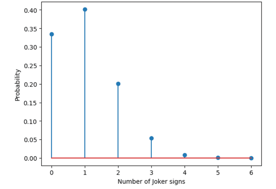
In the SciPy library we have a function called binom.pmf to calculate this with the arguments k equals the number of successes, n equals the number of tries, and p equals the probability for success in a single try. Below is the output for this experiment.

Below is the code for the experiment. You can run it on google colab.

try: #If running in colab
    import google.colab
    IN_COLAB = True
    %tensorflow_version 2.x

except:
    IN_COLAB = False
import tensorflow as tf
if (not tf.__version__.startswith(‘2’)): #Checking if tf 2.0 is installed
    print(‘Please install tensorflow 2.0 to run this notebook’)
print(‘Tensorflow version: ‘,tf.__version__, ‘ running in colab?: ‘, IN_COLAB)

#load required libraries:
import numpy as np
import matplotlib.pyplot as plt
%matplotlib inline
plt.style.use(‘default’)

# Assume a die with only one face with a joker sign
# Calculate probability to observe in 6 throws 1- or 2-times the J-sign
6*(1/6)*(5/6)**5, 15*(1/6)**2*(5/6)**4

from scipy.stats import binom
# Define the numbers of possible successes (0 to 6)
njoker = np.asarray(np.linspace(0,6,7), dtype=’int’)
# Calculate probability to get the different number of possible successes
pjoker_sign = binom.pmf(k=njoker, n=6, p=1/6)
plt.stem(njoker, pjoker_sign)
plt.xlabel(‘Number of Joker signs’)
plt.ylabel(‘Probability’)

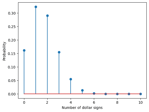
Now consider the following example, you are in a casino and play a game in which you win if a dollar sign appears. You know that there are a certain number of faces (0-6), but you don’t know how many. You observe 10 throws of a die with two dollar signs coming up in those throws. What do you think is the number of dollar signs on the die? By using the code above we can assume that our die this time has two faces with a dollar sign. Our observed data is fixed with ten throws and two dollar signs, but our model changes the data generated from a die with zero dollar faces to a die with 1,2,3…6 dollar faces. The probability of a dollar sign appearing is our parameter. The parameter takes the values p=1/6, 2/6…, 6/6 for our different models. The probability can be determined for each of the models. You can use the code below to calculate the probabilities for each of the models.

try: #If running in colab
    import google.colab
    IN_COLAB = True
    %tensorflow_version 2.x
except:
    IN_COLAB = False

import tensorflow as tf
if (not tf.__version__.startswith(‘2’)): #Checking if tf 2.0 is installed
    print(‘Please install tensorflow 2.0 to run this notebook’)
print(‘Tensorflow version: ‘,tf.__version__, ‘ running in colab?: ‘, IN_COLAB)

#load required libraries:
import numpy as np
import matplotlib.pyplot as plt
%matplotlib inline
plt.style.use(‘default’)

# Assume a die with only one face with a dollar sign
# Calculate the probability to observe in 10 throws 1- or 2-times the $-sign
# See book section 4.1
10*(1/6)*(5/6)**9, 45*(1/6)**2*(5/6)**8

from scipy.stats import binom
# Define the numbers of possible successes (0 to 10)
ndollar = np.asarray(np.linspace(0,10,11), dtype=’int’)
# Calculate the probability to get the different number of possible successes
pdollar_sign = binom.pmf(k=ndollar, n=10, p=1/6) #B
plt.stem(ndollar, pdollar_sign)
plt.xlabel(‘Number of dollar signs’)
plt.ylabel(‘Probability’)

#Solution for model assumption. Different number of dollar signs.
from scipy.stats import binom
#Define the considered numbers of dollar signs on the die (zero to six):
ndollar = np.asarray(np.linspace(0,6,7), dtype=’int’)
#Calculate corresponding probability of 2 $-signs in 10 throws
pdollar = binom.pmf(k=2, n=10, p=ndollar/6)
plt.stem(ndollar, pdollar)
plt.xlabel(‘Number of dollar signs on the dice’)
plt.ylabel(‘Probability observing 2 dollar signs in 10 throws’)
plt.title(‘Unnormalized likelihoods’)

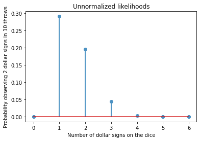
In our example the parametric model is the binomial distribution with two parameters. One parameter is p the probability and the other one is n the number of trials. For our model we chose the p value with the maximum likelihood, p= 1/6. The probabilities shown in the graph above are unnormalized in the sense they do not add up to 1. In the strictest sense they are not probabilities therefore we speak of likelihoods. The likelihoods can be used for ranking and to pick the model with the highest likelihood.

To summarize, for our maximum likelihood approach we need to do the following:

• We need a model for the probability distribution of the data that has one or more parameters. In our example the parameter is probability p.
• We use the model to determine the likelihood to get the observed data when assuming different parameter values.
• The parameter value is chosen for which the likelihood is maximal. This is called the Max-Like estimator. In our model the ML estimator is that the die has one side with a $-sign.

Visit Milton Financial Market Research Institute website to read the next section, Loss functions for classification, and to download the code for the experiment:
https://miltonfmr.com/probabilistic-deep-learning-explained-in-simple-terms/