


![[Gamma] Scalping Please](https://ibkrcampus.com/wp-content/smush-webp/2024/04/tir-featured-8-700x394.jpg.webp "[Gamma] Scalping Please")


This is the second installment of my series on regression analysis used in finance. In the first installment, we touched upon the most important technique in financial econometrics: regression analysis, specifically linear regression and two of its most popular flavours:
- univariate linear regression, and
- multivariate linear regression.
In this post, we apply our knowledge of regression to actual financial data. We will model the relationships from the previous post using Python and R. I run it in both (with downloadable code where applicable) so that readers fluent in one language or application can hopefully get more intuition on its implementation in others.
Many building blocks needed to develop and implement models are available as ready-to-wear software these days. Using them as-is is now standard practice among practitioners of quantitative trading.
Many assumptions underlie the linear regression model. Closely linked to them are also its shortcomings. If you plan to use linear regression for data analysis and forecasting, I’d recommend you look that up first. I intend to write on that topic next.
For now, I shall shrug those worries away and get on with the implementation.
- Implementation using Python
- Implementation using R
Implementation using Python
There are many ways to perform regression analysis in Python. The statsmodels, sklearn, and scipy libraries are great options to work with.
For the sake of brevity, we implement simple and multiple linear regression using the first two.
I point to the differences in approach as we walk through the below code.
We use two ways to quantify the strength of the linear relationship between variables.
- Calculate pairwise correlations between the variables.
- Linear regression modeling (the preferred way).
We start with the necessary imports and get the required financial data.
### Import the required libraries

import numpy as np
import pandas as pd

import yfinance as yf
import datetime
import matplotlib.pyplot as plt

## To use statsmodels for linear regression
import statsmodels.formula.api as smf

## To use sklearn for linear regression
from sklearn.linear_model import LinearRegression
Importing libraries.py hosted with ❤ by GitHub
As discussed in my previous post, we work with the historical returns of Coca-Cola (NYSE: KO), its competitor PepsiCo (NASDAQ: PEP), the US Dollar index (ICE: DX) and the SPDR S&P 500 ETF (NYSEARCA: SPY).
####################################################
## Fetch data from yfinance
## 3-year daily data for Coca-Cola, SPY, Pepsi, and USD index

end1 = datetime.date(2021, 7, 28)
start1 = end1 - pd.Timedelta(days = 365 * 3)

ko_df = yf.download("KO", start = start1, end = end1, progress = False)
spy_df = yf.download("SPY", start = start1, end = end1, progress = False)
pep_df = yf.download("PEP", start = start1, end = end1, progress = False)
usdx_df = yf.download("DX-Y.NYB", start = start1, end = end1, progress = False)

####################################################
## Calculate log returns for the period based on Adj Close prices

ko_df['ko'] = np.log(ko_df['Adj Close'] / ko_df['Adj Close'].shift(1))
spy_df['spy'] = np.log(spy_df['Adj Close'] / spy_df['Adj Close'].shift(1))
pep_df['pep'] = np.log(pep_df['Adj Close'] / pep_df['Adj Close'].shift(1))
usdx_df['usdx'] = np.log(usdx_df['Adj Close'] / usdx_df['Adj Close'].shift(1))

####################################################
Data.py hosted with ❤ by GitHub
####################################################
## Create a dataframe with X's (spy, pep, usdx) and Y (ko)

df = pd.concat([spy_df['spy'], ko_df['ko'],
                pep_df['pep'], usdx_df['usdx']], axis = 1).dropna()

## Save the csv file. Good practice to save data files after initial processing
df.to_csv("Jul2021_data_lin_regression.csv")

####################################################
Dataframe.py hosted with ❤ by GitHub
We first create a scatter plot of the SPY and KO returns to better understand how they are related.
####################################################
## A scatter plot of X (spy) and Y (ko) to examine the nature of their relationship visually

plt.figure(figsize = (10, 6))
plt.rcParams.update({'font.size': 14})
plt.xlabel("SPY returns")
plt.ylabel("KO returns")
plt.title("Scatter plot of daily returns (Jul 2018 to Jul 2021)")
plt.scatter(df['spy'], df['ko'])
plt.show()

####################################################
Scatter Plot.py hosted with ❤ by GitHub
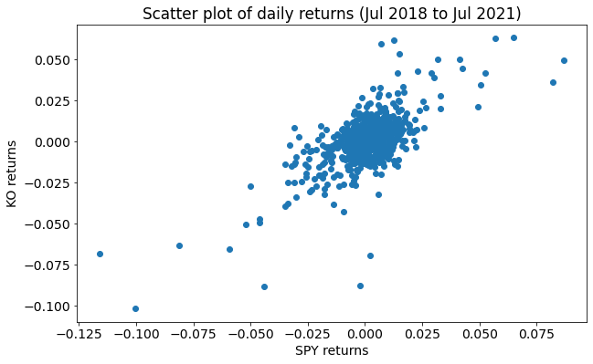
Fig: Scatter plot of daily returns
We also calculate correlations between different variables to analyze the strength of the linear relationships here.
####################################################
## 1. Calculate correlation between Xs and Y

df.corr()

####################################################
Correlation.py hosted with ❤ by GitHub
| spy | ko | pep | usdx | |
|---|---|---|---|---|
| spy | 1.000000 | 0.684382 | 0.725681 | -0.045420 |
| ko | 0.684382 | 1.000000 | 0.738264 | -0.104387 |
| pep | 0.725681 | 0.738264 | 1.000000 | -0.011062 |
| usdx | -0.045420 | -0.104387 | -0.011062 | 1.000000 |
Stay tuned for the next installment in which Vivek Krishnamoorthy will review the statsmodels.
Visit QuantInsti for additional insight on this topic: https://blog.quantinsti.com/linear-regression-market-data-python-r/.
Disclosure: Interactive Brokers
Information posted on IBKR Campus that is provided by third-parties does NOT constitute a recommendation that you should contract for the services of that third party. Third-party participants who contribute to IBKR Campus are independent of Interactive Brokers and Interactive Brokers does not make any representations or warranties concerning the services offered, their past or future performance, or the accuracy of the information provided by the third party. Past performance is no guarantee of future results.
This material is from QuantInsti and is being posted with its permission. The views expressed in this material are solely those of the author and/or QuantInsti and Interactive Brokers is not endorsing or recommending any investment or trading discussed in the material. This material is not and should not be construed as an offer to buy or sell any security. It should not be construed as research or investment advice or a recommendation to buy, sell or hold any security or commodity. This material does not and is not intended to take into account the particular financial conditions, investment objectives or requirements of individual customers. Before acting on this material, you should consider whether it is suitable for your particular circumstances and, as necessary, seek professional advice.