


![[Gamma] Scalping Please](https://ibkrcampus.com/wp-content/smush-webp/2024/04/tir-featured-8-700x394.jpg.webp "[Gamma] Scalping Please")


See Part I and Part II to get started. Visit Robot Wealth to download the complete R script.
How does rsims scale?
Finally, let’s see how rsims performs as we increase the number of time steps and the size of the universe. We’ll benchmark the performance with universe sizes from 100 to 1,000, and time periods from 2,500 to 10,000 days (approximately 10 to 40 trading years):
library(rsims)
get_mean_time <- function(days, universe, times = 5) {
  dates <- seq(as.numeric(as.Date("1980-01-01")), as.numeric(as.Date("1980-01-01"))+(days))
  prices <- cbind(dates, gbm_sim(nsim = universe, t = days, mu = 0.1, sigma = 0.1))
  weights <- cbind(dates, rbind(rep(0, universe), matrix(rnorm(days*universe), nrow = days)))
  res <- microbenchmark(
    cash_backtest(
      prices,
      weights,
      trade_buffer = 0.,
      initial_cash = 1000,
      commission_pct = 0.001,
      capitalise_profits = FALSE
    ),
    times = times
  )
  mean(res$time)/1e9
}
num_assets <- seq(100, 1000, 100)
num_days <- c(10, 20, 30, 40)*252
means <- list()
for(universe in num_assets) {
  print(glue::glue("Doing universe size {universe}"))
  for(days in num_days) {
    print(glue::glue("Doing {days} days"))
    means <- c(means, get_mean_time(days, universe, times = 10))
  }
}
Plotting the results:
df <- as.data.frame(matrix(unlist(means), ncol = length(num_assets))) %>%
  mutate(days = num_days)
colnames(df) <- c(num_assets, "days")
df %>%
  pivot_longer(cols = -days, names_to = "universe_size", values_to = "mean_sim_time") %>%
  mutate(universe_size = as.numeric(universe_size)) %>%
  ggplot(aes(x = universe_size, y = mean_sim_time, colour = factor(days))) +
    geom_line() +
    geom_point() +
    labs(
      x = "Universe size",
      y = "Mean simulation time, seconds",
      title = "Mean simulation time from 10 iterations",
      colour = "Time Steps"
    ) +
    theme_bw()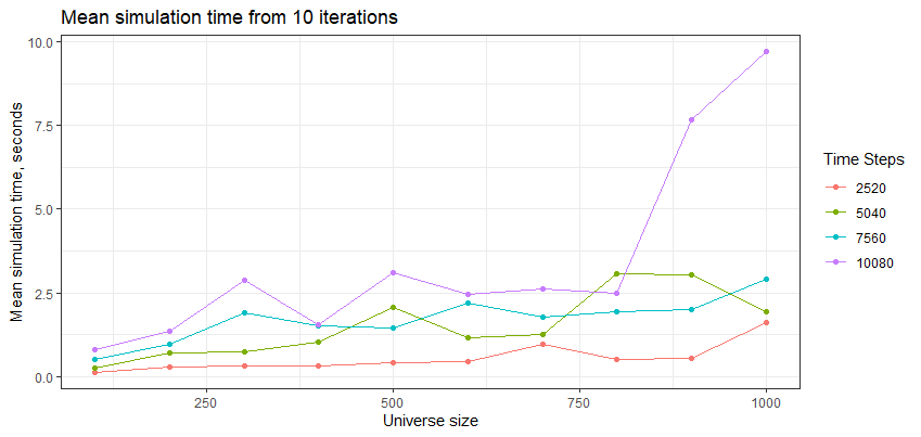
We can see that rsims scales well in general. I suspect that there was a blow out for the universe sizes of 900 and 1,000 for the 40-year backtest due to memory constraints of my local setup (100 Chrome tabs anyone?).
Other ideas not implemented
There are some other tricks for speeding up R code that weren’t applicable here, but that are worth knowing about.
Parallel processing
Parallel processing is a well-trodden path for doing computations in parallel on more than one processor. In R, the parallel package is the original parallel processing toolkit and is included in base R. It parallelises some standard R functions out of the box, such as the apply functions. There’s also the foreach and doParallel packages.
In our application, parallelisation won’t work for the event loop because of path dependency – tomorrow’s trades depend on yesterday’s positions, so we can’t do yesterday’s and today’s trades in parallel.
We could potentially parallelise the position delta calculations for each asset within each loop iteration, as these aren’t dependent on one another. This operation is already fast – on the order of microseconds – so we have little to gain in absolute terms, and I think the overhead of setting up and managing parallel processes would probably negate any speed gains anyway.
Intelligent application of logical operators
A common inefficiency is using vectorised AND and OR operators (&, |) in comparisons involving scalars. The vectorised versions always evaluate both sides of the logical operator, whereas the non-vectorised versions (&&, ||) only execute the right-hand side (and subsequent comparisons) if necessary.
For example, the expression (1 > 4) & (3 < 5) evaluates both sides of the &, while (1 > 4) && (3 < 5) only evaluates the first, because the expression is falsified by the first comparison.
Granted, this is a very minor inefficiency but can make a difference if you’re doing a lot of such operations. Just be careful not to use scalar && and || on vectors, as they will only evaluate the first element!
Conclusion
By far the biggest efficiency gains came with converting data frames to matrixes. This is worth considering when speed is important, so long as the trade-offs around data consistency and convenience make sense for the application.
Smaller but useful efficiency gains came from:
- Preallocating data containers rather than growing them on the fly
- Pushing data transformations that only need to happen once outside the function whose speed matters (for example, make the wide price and weights matrixes once, then run many fast backtests with different parameters)
- Vectorising where possible
- Using C++ via
Rcpp
You might also want to consider parallel processing and careful usage of logical operators.
Disclosure: Interactive Brokers
Information posted on IBKR Campus that is provided by third-parties does NOT constitute a recommendation that you should contract for the services of that third party. Third-party participants who contribute to IBKR Campus are independent of Interactive Brokers and Interactive Brokers does not make any representations or warranties concerning the services offered, their past or future performance, or the accuracy of the information provided by the third party. Past performance is no guarantee of future results.
This material is from Robot Wealth and is being posted with its permission. The views expressed in this material are solely those of the author and/or Robot Wealth and Interactive Brokers is not endorsing or recommending any investment or trading discussed in the material. This material is not and should not be construed as an offer to buy or sell any security. It should not be construed as research or investment advice or a recommendation to buy, sell or hold any security or commodity. This material does not and is not intended to take into account the particular financial conditions, investment objectives or requirements of individual customers. Before acting on this material, you should consider whether it is suitable for your particular circumstances and, as necessary, seek professional advice.