Price Action Trading Concepts – Part III

See Part I for an overview of price action trading and the different types of charts and Part II to get insight on the concept of support and resistance.

Identifying support and resistance using Python

The first step in our approach is to import necessary libraries and get the asset data.

We will be focusing on the close price data of HINDUNILVR.NS for performing the support and resistance analysis. We fetch the asset’s OHLCV data from Yahoo! Finance and store it in a dataframe as shown below.

# Import Libraries
import numpy as np
import pandas as pd
import yfinance as yf
from math import sqrt
import matplotlib.pyplot as plt

# Set the start and end date
start = '2018-01-01°
end = ‘2021-07-12

# Set the ticker
symbol = "HINDUNTLVR.NS*

# Get the data from Yahoo! Finance
df = yf.dounload(symbol, start, end)

# Disply the data
df.tail()

Fetch data.py hosted with ❤ by GitHub

The last 5 rows of our data can be displayed using the df.tail() command.

Output:

Date	Open	High	Low	Close	Adj Close	Volume
2021-07-05	2499.000000	2513.399902	2485.050049	2499.050049	2499.050049	761700
2021-07-06	2490.000000	2497.949951	2469.000000	2472.500000	2472.500000	461782
2021-07-07	2458.000000	2490.800049	2445.850098	2481.649902	2481.649902	623145
2021-07-08	2462.199951	2469.750000	2438.449951	2447.550049	2447.550049	1114426
2021-07-09	2440.000000	2464.500000	2438.449951	2451.449951	2451.449951	538094

To get a visual representation of the close price data, we will use various functions of the matplotlib library.

# Plot the close price data
series = df[‘Close’]
series. index = np.arange(series.shape[@])

plt. figure(figsize=(15, 7))
plt.title(symbol)

plt.xlabel ("Days")
plt.ylabel("Price’)
plt.plot(series, label-symbol)

plt.legend()
plt.show()

Plot.py hosted with ❤ by GitHub

Here’s the graph highlighting the close price of the asset:

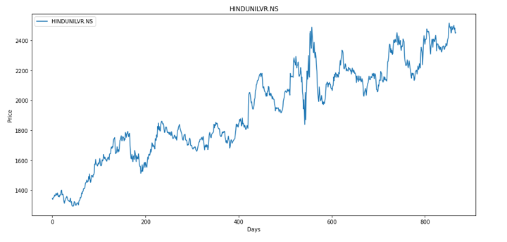
Close price

Now since we have all our data in place, the next step is to identify the swing highs and the swing lows in the above price graph. An easier way to do this is to identify the local minima and local maxima points.

To identify the local minima and maxima points, we will first need to smoothen the price graph. This can be achieved using the savgol.filter function from the scipy.signal library. To learn more about this function, you can visit the documentation page here.

# Create smooth graph of close price data
from scipy.signal import savgol_filter

# To find amount of data in months
month_diff = series.shape[0] // 30
# We need value to be greater than 0
if month_diff == 0:
    month_diff = 1

# Algo to determine smoothness
smooth = int(2 * month diff + 3)

# Smooth price data
points = savgol_filter(series, smooth, 7)

# Plot the smooth price graph over default price graph
plt. figure(figsize=(15,7))

plt.title(symbol)

plt.xlabel ("Days")

plt.ylabel("Price’)

# Close price data
plt.plot(series, label-symbol)

# Smooth close price data
plt.plot(points, label=f'Smooth {symbol}")

plt.legend()
plt.show()

Smooth graph.py hosted with ❤ by GitHub

Stay tuned for the next installment of this series to learn how to plot and compare the normal close price graph with the smoothened close price graph

For additional insight on this topic visit QuantInsti blog: https://blog.quantinsti.com/price-action-trading/.