QuantConnect Idea Streams #2 – Modeling Unemployment Rates with SKLearn

The article “Idea Streams #2 – Modeling Unemployment Rates with SKLearn” first appeared on QuantConnect. The below is an excerpt. To watch Jared Broad’s presentation on this topic visit QuantConnect.

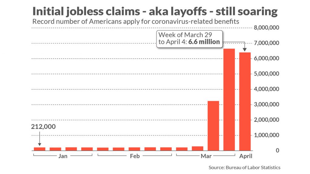
Before the coronavirus hit, the US unemployment rate was at a 50-year low of 3.5%. Then in April 2020, Reuters reported that the US unemployment rate would likely rise to 16% in the next jobs report, a rate approaching the levels seen in the 1930s. In addition to these figures, MarketWatch reported an unprecedented spike in unemployment insurance claims. They noted that “just a month ago, new claims were in the low 200,000s and sat near a half-century low,” but new claims quickly jumped to 6-7 million per week.

In response to these unusual figures, we wanted to test if there is some sort of factor in these data sets that we could tie to the overall US stock market. So in Idea Streams episode #2, we took a look at how the US unemployment rate and the number of unemployment insurance claims influenced the prices of some market indices.

Our Process

Our analysis started by gathering the Unemployment Rate and Initial Claims datasets from the Federal Reserve Economic Database. To import these into our research environment, we created two custom data readers. We noticed the timestamps in the datasets from FRED were set to the beginning of each period. That is, the unemployment rate for March 2020 wasn’t reported until April 3rd. When it was reported, the data point was timestamped as March 2020. To remove lookahead bias, we designed the custom data readers to move the timestamps forward to approximately the date when the data point would have been reported.

With the data now timestamped to the reporting date, we continued our analysis by training a linear regression model to anticipate the price of SPY using each of the individual data sets from FRED. We trained the models using all of the data points except the last 5. The last 5 data points were saved to test the models out-of-sample. Training and testing the regression models produced the following results.

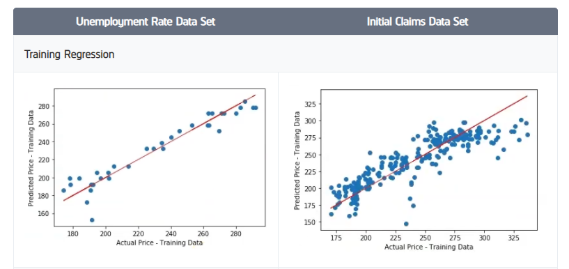
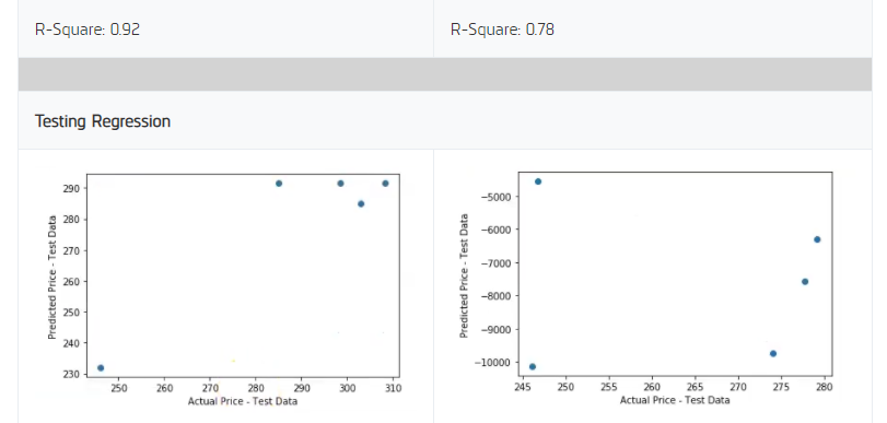
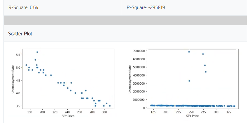
We saw a higher R-Square on the training data set when using the unemployment rate dataset. The last 5 data points for the employment insurance claims data set were way off the record of what anyone has seen before, so it’s not unexpected that the model produces such a low R-Square value. With the unemployment rate having a higher R-Square value, we select this data set to continue our analysis.

Up until this point, we’ve been using SPY price as the dependent variable in our regression. The articles that inspired this strategy mentioned that the broader market is being held up by AAPL, MSFT, and a few large tech companies. The idea is that larger companies with more cash on their balance sheets would be better handled to weather a recession, so investors might have a “flight to safety”, moving out of stocks that have a relatively worse-off position and into stocks that have a relatively stronger position.

We tested this theory by looking at the latest drawdowns of a large tech company (AAPL), the overall market index (SPY), and a small-cap index (VB). We found the following drawdowns:

• AAPL – 13.8%
• SPY – 15.4%
• VB – 24.1%

In light of this finding, we replaced SPY with VB, retrained the regression model, and found the following R-squared values:

• In-sample: 0.87
• Out-of-sample: 0.78

We also noticed that the R-square values here were quite sensitive to the adjusted timestamp in the custom data. To get the most realistic results, the actual reporting date of each data point would need to be gathered. Regardless, we deemed our R-square value good enough to continue our experiment with a backtest.

Results

VB was listed in 2004, so we set the start date of the backtest to January 1, 2005, allowing us to run the strategy through the 2008 crash. The strategy rules are simple: if the unemployment rate is increasing, be invested in VB; otherwise, exit the market until it gets better. Backtesting the strategy resulted in a 44.5% drawdown, a 0.349 Sharpe ratio, and a flat equity curve during the 2008 crash. In contrast, buying and holding VB during the same time period resulted in a 59.6% drawdown and a 0.379 Sharpe ratio. Therefore, in conclusion, using the strategy resulted in a better drawdown but a worse Sharpe ratio.

Visit QuantConnect to read the full article and watch Jared Broad’s presentation on this topic: https://www.quantconnect.com/blog/idea-streams-2-modeling-unemployment-rates-with-sklearn/.

QuantConnect aims to provide an opportunity for a diverse community of brilliant thinkers to learn, show off their skills and do fulfilling work. We nurture a global community of quantitative engineers to build algorithms and contribute to the LEAN code base. The community shapes the technology design and helps bring the project to fruition in our open-source, decentralized, hybrid-cloud environment.