Sign Constrained Lasso with R code

This post explains how to implement the sign constrained lasso with ridge, and linear regression model. The restrictions of expected sign is of great importance in the case when building an econometric model with meaningful interpretation. We can easily incorporate sign restrictions to the above regression models using glmnet R package.

It is a stylized fact that the default risk decreases in GDP growth rate, but increase in GDP growth volatility. This relationship is empirical and theoretical guideline for the model selection. Therefore, all explanatory variables should be consistent to its own expected signs.

The lasso, ridge, and linear regression model is the unrestricted model as default setting. But The sign restrictions need to be included as additional constraints in optimization problem. Implementing this optimization problem is not easy but we can sidestep this difficulty by using glmnet R package.

Since the following R code have a self-contained structure, it is easy to understand. In this code, The expected signs of each coefficients are given by user as following rule.

•  1 : expected sign is plus(+)
• -1 : expected sign is mimus(-)
•  0 : expected sign is indeterminate

#===================================================================#
# Financial Econometrics & Derivatives, ML/DL, R,Python,Tensorflow 
# by Sang-Heon Lee
#
# https://kiandlee.blogspot.com
#-------------------------------------------------------------------#
# Sign constrained Lasso, Ridge, Stnadard Linear Regression
#===================================================================#
 
library(glmnet)
 
    graphics.off()  # clear all graphs
    rm(list = ls()) # remove all files
    
    N = 500 # number of observations
    p = 20  # number of variables
    
#--------------------------------------------
# X variable
#--------------------------------------------
    X = matrix(rnorm(N*p), ncol=p)
 
    # before standardization
    colMeans(X)    # mean
    apply(X,2,sd)  # standard deviation
 
    # scale : mean = 0, std=1
    X = scale(X)
 
    # after standardization
    colMeans(X)    # mean
    apply(X,2,sd)  # standard deviation
 
#--------------------------------------------
# Y variable
#--------------------------------------------
    beta = c( 0.15, -0.33,  0.25, -0.25, 0.05,
              rep(0, p/2-5), -0.25,  0.12, -0.125, 
              rep(0, p/2-3))
 
    # Y variable, standardized Y
    y = X%*%beta + rnorm(N, sd=0.5)
    y = scale(y)
 
#--------------------------------------------
# Model without Sign Restrictions
#--------------------------------------------
    
    # linear regression without intercept( using -1)
    li.eq <- lm(y ~ X-1) 
    
    # linear regression using glmnet
    li.gn <- glmnet(X, y, lambda=0, family="gaussian", 
                    intercept = F, alpha=0) 
    # lasso
    la.eq <- glmnet(X, y, lambda=0.05, family="gaussian", 
                    intercept = F, alpha=1) 
    # Ridge
    ri.eq <- glmnet(X, y, lambda=0.05, family="gaussian", 
                    intercept = F, alpha=0) 
    
#--------------------------------------------
# Model with Sign Restrictions
#--------------------------------------------
    
    # Assign Expected sign as arguments of glmnet
    v.sign <- sample(c(1,0,-1),p,replace=TRUE)
    vl <- rep(-Inf,p); vu <- rep(Inf,p)
    
    for (i in 1:p) {
        if      (v.sign[i] ==  1) vl[i] <- 0 
        else if (v.sign[i] == -1) vu[i] <- 0 
    }
    
    # linear regression using glmnet with sign restrictions
    li.gn.sign <- glmnet(X, y, lambda=0, family="gaussian", 
                     intercept = F, alpha=1, 
                     lower.limits = vl, upper.limits = vu) 
    # lasso with sign restrictions
    la.eq.sign <- glmnet(X, y, lambda=0.05, family="gaussian",
                     intercept = F, alpha=1, 
                     lower.limits = vl, upper.limits = vu) 
    # Ridge with sign restrictions
    ri.eq.sign <- glmnet(X, y, lambda=0.05, family="gaussian", 
                     intercept = F, alpha=0, 
                     lower.limits = vl, upper.limits = vu) 
 
#--------------------------------------------
# Results
#--------------------------------------------
    df.out <- as.data.frame(as.matrix(round(
              cbind(li.eq$coefficients, 
                    li.gn$beta, li.gn.sign$beta,
                    la.eq$beta, la.eq.sign$beta, 
                    ri.eq$beta, ri.eq.sign$beta),4)))
    # for clarity
    df.out[df.out==0] <- "."
    df.out <- cbind(
       ifelse(v.sign==1,"+",ifelse(v.sign==-1,"-",".")),
       ifelse(v.sign==1,"plus",ifelse(v.sign==-1,"minus",".")),
       df.out)
    # always important to use appropriate column names
    colnames(df.out) <- c("Sign", "Desc", "Linear.lm", 
        "Linear", "Linear.Sign","Lasso", "Lasso.Sign",
        "Ridge", "Ridge.Sign")
    print(df.out)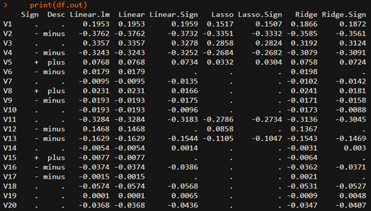

From the above estimation results, we can find that estimated coefficients are consistent with each expected sign. When estimated sing conflicts with the expected one, its coefficients is set to zero and is discarded. Therefore we can understand that the sign restrictions is another form of variable selection process which reduce more the range of selected variables.

Generally speaking, it is not easy to impose the expected sign restrictions but we can do it with powerful glmnet R package.

For additional insight on this topic and to download the R script, visit the SH Fintech Modeling Blog.