Sklearn – An Introduction Guide to Machine Learning

The article “Sklearn – An Introduction Guide to Machine Learning” first appeared on AlgoTrading101 Blog.

Excerpt

What is Sklearn?

Sklearn (scikit-learn) is a Python library that provides a wide range of unsupervised and supervised machine learning algorithms.

It is also one of the most used machine learning libraries and is built on top of SciPy.

What is Sklearn used for?

The Sklearn Library is mainly used for modeling data and it provides efficient tools that are easy to use for any kind of predictive data analysis.

The main use cases of this library can be categorized into 6 categories which are the following:

• Preprocessing
• Regression
• Classification
• Clustering
• Model Selection
• Dimensionality Reduction

As this article is mainly aimed at beginners, we will stick to the core concepts of each category and explore some of its most popular features and algorithms.

Advanced readers can use this article as a recollection of some of the main use cases and intuitions behind popular sklearn features that most ML practitioners couldn’t live without.

Each category will be explained in a beginner-friendly and illustrative way followed by the most used models, the intuition behind them, and hands-on experience. But first, we need to set up our sklearn library.

How to download Sklearn for Python?

Sklearn can be obtained in Python by using the pip install function as shown below:

$ pip install -U scikit-learn

Sklearn developers strongly advise using a virtual environment (venv) or a conda environment when working with the library as it helps to avoid potential conflicts with other packages.

How to pick the best Sklearn model?

When it comes to picking the best Sklearn model, there are many factors that come into play that range from experience and data to the problem scope and math behind each algorithm.

Sometimes all chosen algorithms can have similar results and, depending on the problem setting, you will need to pick the one that is the fastest or the one that generalizes the best on big data.

It may happen that all of your promised models won’t perform well enough and that you will simply need to combine multiple models (e.g. ensemble), make your own custom-made model, or go for a deep learning approach.

As picking the right model is one of the foundations of your problem solving, it is wise to read-up on as many models and their uses as you can.

As model selection would be an article, or even a book, for itself, I’ll only provide some rough guidelines in the form of questions that you’ll need to ask yourself when deciding which model to deploy.

How much data do you have?

Some models are better on smaller datasets while others require more data and tend to generalize better on larger datasets (e.g. SGD Regressor vs Lasso Regression).

What are the main characteristics of your data?

Is your data linear, quadratic, or all over the place? How do your distributions look like? Is your data made out of numbers or strings? Is the data labeled?

What kind of a problem are you solving?

Are you trying to predict: which cat will push most jars of the table, is that a dog or a cat, or of which dog breeds are a group of dogs made up?

All of these questions have different approaches and solutions. Thus we will explore later in the article the three main problem classifications:

• regression
• classification
• clustering

How do your models perform when compared against each other?

You will see that scikit-learn comes equipped with functions that allow us to inspect each model on several characteristics and compare it to the other ones.

Take note that scikit-learn has created a good algorithm cheat-sheet that aids you in your model selection and I’d advise having it near you at those troubling times.

Sklearn preprocessing – Prepare the data for analysis

When you think of data you probably have in mind a ginormous excel spreadsheet full of rows and columns with numbers in them. Well, the case is that data can come in a plethora of formats like images, videos and audio.

The main job of data preprocessing is to turn this data into a readable format for our algorithm. A machine can’t just “listen in” to an audiotape to learn voice recognition, rather it needs it to be converted numbers.

The main building blocks of our dataset are called features which can be categorical or numerical. Simply put, categorical data is used to group data with similar characteristics while numerical data provides information with numbers.

As the features come from two different categories, they need to be treated (preprocessed) in different ways. The best way to learn is to start coding along with me.

Sklearn feature encoding

Feature encoding is a method where we transform categorical variables into continuous ones. The most popular ways of doing so are known as One Hot Encoding and Label encoding.

For example, a person can have features such as [“male”, “female], [“from US”, “from UK”], [“uses Binance”, “uses Coinbase”]. These features can be encoded as numbers e.g. [“male”, “from US”, “uses Coinbase”] would be [0, 0, 1].

This can be done by using the scikit-learn OrdinalEncoder() function as follows:

pip install scikit-learn
from sklearn import preprocessing

X = [['male', 'from US', 'uses Coinbase'], ['female', 'from UK', 'uses Binance']]
encode = preprocessing.OrdinalEncoder()
encode.fit(X)

encode.transform([['male', 'from UK', 'uses Coinbase']])

Output: array([[1., 0., 1.]])

As you can see, it transformed the features into integers. But they are not continuous and can’t be used with scikit-learn estimators. In order to fix this, a popular and most used method is one hot encoding.

One hot encoding, also known as dummy encoding, can be obtained through the scikit-learn OneHotEncoder() function. It works by transforming each category with N possible values into N binary features where one category is represented as 1 and the rest as 0.

The following example will hopefully make it clear:

one_hot = preprocessing.OneHotEncoder()
one_hot.fit(X)

one_hot.transform([['male', 'from UK', 'uses Coinbase'],
                   ['female', 'from US', 'uses Binance']]).toarray()

Output: array([[0., 1., 1., 0., 0., 1.],
              [1., 0., 0., 1., 1., 0.]])

To see what your encoded features are exactly you can always use the .categories_ attribute as shown below:

one_hot.categories_

Output: [array(['female', 'male'], dtype=object),
         array(['from UK', 'from US'], dtype=object),
         array(['uses Binance', 'uses Coinbase'], dtype=object)]

Sklearn data scaling

Feature scaling is a preprocessing method used to normalize data as it helps by improving some machine learning models. The two most common scaling techniques are known as standardization and normalization.

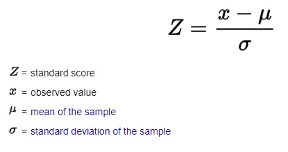
Standardization makes the values of each feature in the data have zero-mean and unit variance. This method is commonly used with algorithms such as SVMs and Logistic regression.

Standardization is done by subtracting the mean from each feature and dividing it by the standard deviation. It’s some basic statistics and math, but don’t worry if you don’t get it. There are many tutorials that cover it.

In scikit-learn we use the StandardScaler() function to standardize the data. Let us create a random NumPy array and standardize the data by giving it a zero mean and unit variance.

import numpy as np

scaler = preprocessing.StandardScaler()
X = np.random.rand(3,4)
X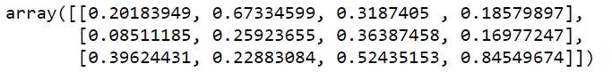

X_scaled = scaler.fit_transform(X)
X_scaled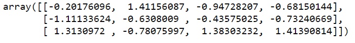

print(f'The scaled mean is: {X_scaled.mean(axis=0)}nThe scaled variance is: {X_scaled.std(axis=0)}')

Wait for a second! Didn’t you say that all mean values need to be 0?

Well, in practice these values are so close to 0 that they can be viewed as zero. Moreover, due to limitations with numerical representations the scaler can only get the mean really close to a zero.

Let’s move onto the next scaling method called normalization. Normalization is a term with many definitions that change from one field to another and we are going to define it as follows:

Normalization is a scaling technique in which values are shifted and rescaled so that they end up being between 0 and 1. It is also known as Min-Max scaling. In scikit-learn it can be applied with the Normalizer() function.

norm = preprocessing.Normalizer()

X_norm = norm.transform(X)
X_norm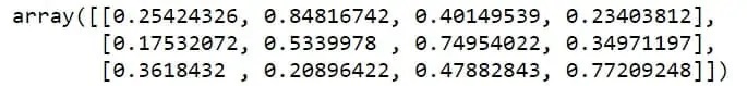

So, which one is better? Well, it depends on your data and the problem you’re trying to solve. Standardization is often good when the data is depicting a Normal distribution and vice versa. If in doubt, try both and see which one improves the model.

Sklearn missing values

In scikit-learn we can use the .impute class to fill in the missing values. The most used functions would be the SimpleImputer(), KNNImputer() and IterativeImputer().

When you encounter a real-life dataset it will 100% have missing values in it that can be there for various reasons ranging from rage quits to bugs and mistakes.

There are several ways to treat them. One way is to delete the whole row (candidate) from the dataset but it can be costly for small to average datasets as you can delete plenty of data.

Some better ways would be to change the missing values with the mean or median of the dataset. You could also try, if possible, to categorize your subject into their subcategory and take the mean/median of it as the new value.

Let’s use the SimpleImputer() to replace the missing value with the mean:

from sklearn.impute import SimpleImputer

imputer = SimpleImputer(missing_values=np.nan, strategy="mean")
imputer.fit_transform([[10,np.nan],[2,4],[10,9]])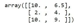

The strategy hyperparameter can be changed to median, most_frequent, and constant. But Igor, can we impute missing strings? Yes, you can!

import pandas as pd

df = pd.DataFrame([['i', 'g'],
                   ['o', 'r'],
                   ['i', np.nan],
                   [np.nan, 'r']], dtype='category')

imputer = SimpleImputer(strategy='most_frequent')
imputer.fit_transform(df)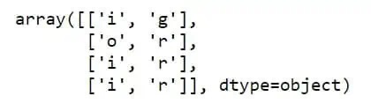

If you want to keep track of the missing values and the positions they were in, you can use the MissingIndicator() function:

from sklearn.impute import MissingIndicator

# Image the 3's were imputed by the SimpleImputer()
Y = np.array([[3,1], 
              [5,3],
              [9,4], 
              [3,7]])

missing = MissingIndicator(missing_values=3)
missing.fit_transform(Y)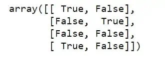

The IterateImputer() is fancy, as it basically goes across the features and uses the missing feature as the label and other features as the inputs of a regression model. Then it predicts the value of the label for the number of iterations we specify.

If you’re not sure how regression algorithms work, don’t worry as we will soon go over them. As the IterativeImputer() is an experimental feature we will need to enable it before use:

from sklearn.experimental import enable_iterative_imputer
from sklearn.impute import IterativeImputer

imputer = IterativeImputer(max_iter=15, random_state=42)
imputer.fit_transform(([1,5],[4,6],[2, np.nan], [np.nan, 8]))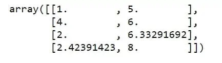

Sklearn train test split

In Sklearn the data can be split into test and training groups by using the train_test_split() function which is a part of the model_selection class.

But why do we need to split the data into two groups? Well, the training data is the data on which we fit our model and it learns on it. In order to evaluate how the model performs on unseen data, we use test data.

An important thing, in most cases, is to allocate more data to the training set. When speaking of the ratio of this allocation there aren’t any hard rules. It all depends on the size of your dataset.

The most used allocation ratio is 80% for training and 20% for testing. Have in mind that most people use the training/development set split but name the dev set as the test set. This is more of a conceptual mistake.

Now let us create a random dataset and split it into training and testing sets:

from sklearn.datasets import make_blobs
from sklearn.model_selection import train_test_split

# Create a random dataset
X, y = make_blobs(n_samples=1500)

# Split the data
X_train, X_test, y_train, y_test = train_test_split(X, y, test_size=0.20)

print(f'X training set {X_train.shape}nX testing set {X_test.shape}ny training set {y_train.shape}ny testing set {y_test.shape}')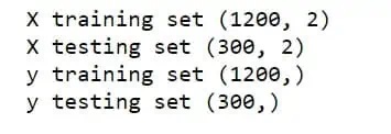

If your dataset is big enough you’ll often be fine with using this way to split the data. But some datasets come with a severe imbalance in them.

For example, if you’re building a model to detect outliers that default their credit cards you will most often have a very small percentage of them in your data.

This means that the train_test_split() function will most likely allocate too little of the outliers to your training set and the ML algorithm won’t learn to detect them efficiently. Let’s simulate a dataset like that:

from sklearn.datasets import make_classification
from collections import Counter

# Create an imablanced dataset
X, y = make_classification(n_samples=1000, weights=[0.95], flip_y=0, random_state=42)
print(f'Number of y before splitting is {Counter(y)}')

# Split the data the usual way
X_train, X_test, y_train, y_test = train_test_split(X, y, test_size=0.20, random_state=42)
print(f'Number of y in the training set after splitting is {Counter(y_train)}')
print(f'Number of y in the testing set after splitting is {Counter(y_test)}')

As you can see, the training set has 43 examples of y while the testing set has only 7! In order to combat this, we can split the data into training and testing by stratification which is done according to y.

This means that y examples will be adequately stratified in both training and testing sets (20% of y goes to the test set). In scikit-learn this is done by adding the stratify argument as shown below:

# Split the data by stratification
X_train, X_test, y_train, y_test = train_test_split(X, y, test_size=0.20, stratify=y, random_state=42)
print(f'Number of y in the training set after splitting is {Counter(y_train)}')
print(f'Number of y in the testing set after splitting is {Counter(y_test)}')

For a more in-depth guide and understanding of the train test split and cross-validation, please visit the following article that is found on our blog: https://algotrading101.com/learn/train-test-split/

For more information about scikit-learn preprocessing functions go here.

Visit AlgoTrading101 to read the rest of the article.