Trend-Following Filters – Part 5

The article “Trend-Following Filters – Part 5” first appeared on Alpha Architect Blog.

Excerpt

1. Introduction

Previous articles in this series examine, from a digital signal processing (DSP) frequency domain perspective, various types of digital filters used by quantitative analysts and market technicians to analyze and transform financial time series for trend-following purposes.

1. An Introduction to Digital Signal Processing for Trend Following
2. Trend-Following Filters – Part 1
3. Trend-Following Filters – Part 2
4. Trend-Following Filters – Part 3
5. Trend-Following Filters – Part 4

Part 4 of this series, along with this article, examines the application of the Kalman filter to financial time series. The Kalman filter is a statistics-based algorithm used to perform estimation of random processes⁽¹⁾. Estimation of processes in noisy environments is a critical task in many fields, such as communications, process control, track-while-scan radar systems, robotics, and aeronautical, missile, and space vehicle guidance. The Kalman filter is a real-time algorithm that operates iteratively in the discrete-time domain and is used in a variety of complex random process estimation applications.

There are two general types of Kalman filter models: steady-state and adaptive. A steady-state filter assumes that the statistics of the process under consideration are constant over time, resulting in fixed, time-invariant filter gains. The gains of an adaptive filter, on the other hand, are able to adjust to processes that have time-varying dynamics, such as financial time series which typically display volatility and non-stationarity.

2. Two State Noise-Adaptive Kalman Filter

This article assumes familiarity with Part 4, which includes an overview of the Kalman filter and describes an adaptive covariance matching method originally proposed by Myers and Tapley ⁽²⁾ and re-stated with some modification by Stengel ⁽³⁾. The Stengel version is employed in both articles. The method estimates the process and measurement noise covariances directly from the Kalman filter algorithm, replacing, for example, the need for assumed or externally-derived noise covariance estimates.

To more easily illustrate adaptive filter concepts and calculations, the Kalman filter algorithm described in Part 4 has one state variable, x(t), modeled on a first-order process that has a locally constant mean value a contaminated by additive random noise ε(t)^~N(0, σ_ε²):

y(t) = a + ε(t)

The filter described in this article has two state variables, x₁(t) and x₂(t), modeled on a second-order process that has mean value a and locally constant linear trend b contaminated by additive random noise:

y(t) = a + b*t + ε(t)

More specifically, the process models in both articles are based on the assumption that financial asset prices follow the general Newtonian equation of motion ⁽⁴⁾:

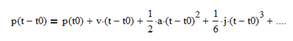
where p is the position (analogous to a financial asset price), v is the velocity (analogous to what is commonly called “momentum” by quantitative analysts and market technicians), a is the acceleration (change in velocity), j is the jerk (change in acceleration), etc. State variable x₁(t) is equivalent to the second-order process mean value a as well as to Newtonian position p. State variable x₂(t) is equivalent to second-order process linear trend b as well as to Newtonian velocity v (i.e., it is assumed that acceleration a = 0, jerk j = 0, etc.).

The two-state noise-adaptive Kalman filter process and measurement model equations, variable initialization, algorithm steps, and noise estimate calculations are shown in Appendix 1 where:

• the number of state variables n = 2,
• the two state variables are position x₁(t) and velocity x₂(t),
• the number of measurements m = 1 since only position (i.e., price) measurements z(t) are assumed to be available,
• the time step is 1 trading day,
• since the Newtonian motion equations that include only position p and velocity v are p(t) = p(t-1) + v*Δt and v(t) = v(t-1), respectively, the state transition matrix is:

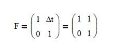
where Δt = 1-time step

• the process noise inputs g₁ = ½ and g₂ = 1, based on the process model assumption that the velocity is locally constant and subject to random acceleration noise ⁽⁵⁾,
• the state measurement input vector H = (1 0) since only position is measured,
• the filter gains k₁(t) and k₂(t) range between 0 and 1, and
• the number of process and measurement noise samples N in the sliding time window is 10 trading days.

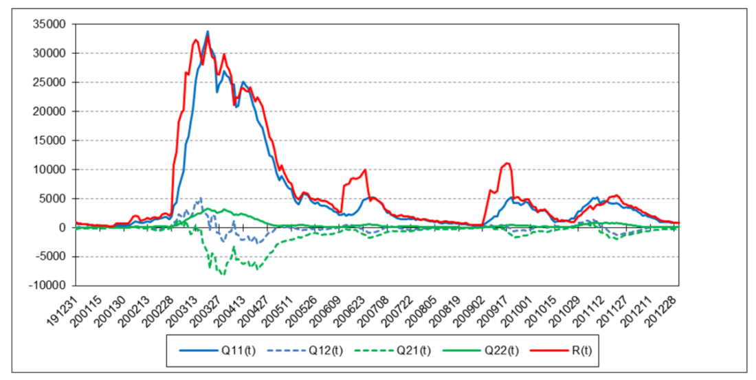
The noise-adaptive method estimates the measurement and process noise covariances simultaneously with the state estimates. Since only measurements z(t) of position are available, the noise-adaptive method uses a set of measurement noise samples r(t), also called “residuals”, where:

r(t) = z(t) – x₁^–(t)

made over a sliding time window of length N time steps (N > 1) to estimate the measurement noise mean r’(t) and variance R(t). That is, the most recent set of N noise samples made over time steps t-N+1 to t is used in the calculations at each time step t. It uses sets of approximate position and velocity process noise samples q₁(t) and q₂(t), respectively, where:

q₁(t) = [x₁⁺(t) – (x₁⁺(t-1) + x₂⁺(t-1))] / g₁

q₂(t) = [x₂⁺(t) – x₂⁺(t-1)] / g₂

and g₁ and g₂ are the position and velocity process noise input scalars, respectively, made over the sliding time window to estimate the process noise means q₁’(t) and q₂’(t) and covariances Q₁₁(t), Q₁₂(t), Q₂₁(t), and Q₂₂(t). The measurement and process noise means and covariances are re-estimated each time the window is shifted forward by one time step.

3. Two State Noise-Adaptive Kalman Filter Examples

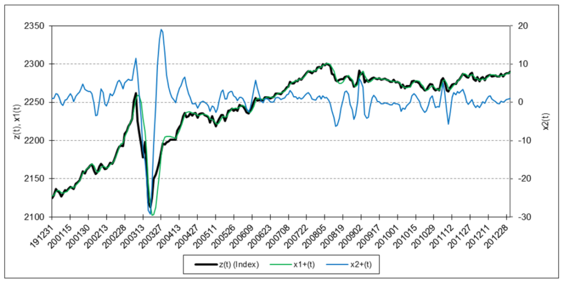
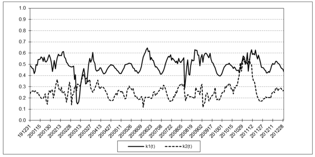
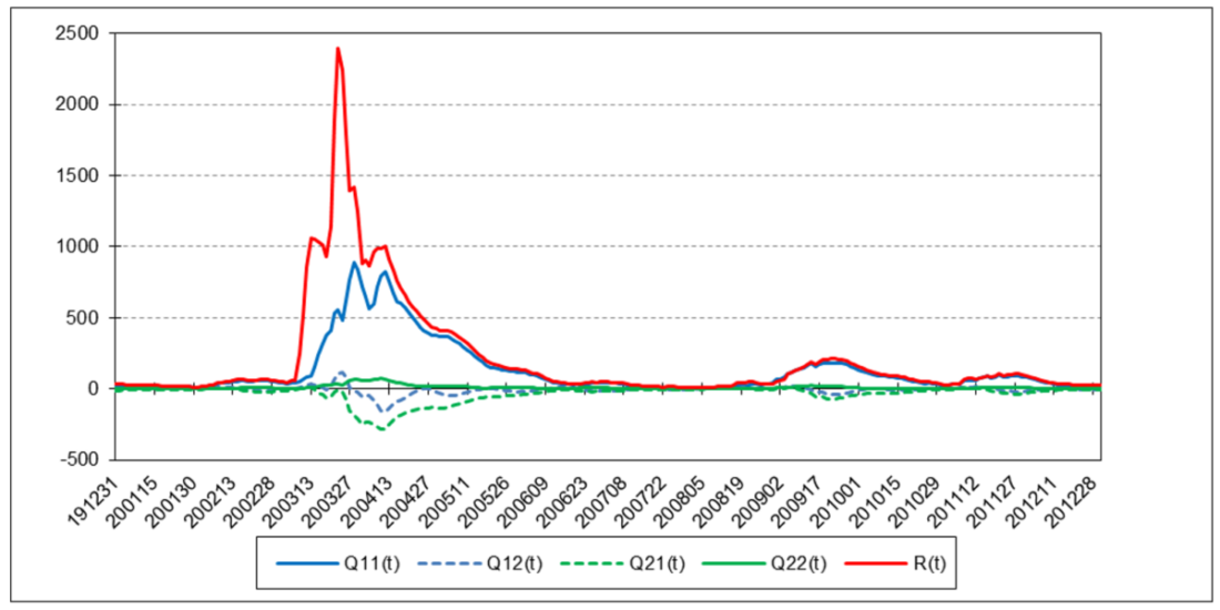
The following charts illustrate the application of the two-state noise-adaptive Kalman filter method to the daily closing values of a stock index, a bond index, a currency, a commodity index, and a volatility index for the year 2020. The upper chart of each example shows the index or FX rate input z(t) and the state estimate measurement update outputs x₁⁺(t) and x₂⁺(t), the middle chart shows the filter gains k₁(t) and k₂(t), and the lower chart shows the associated Q(t) and R(t) covariances.

S&P 500 Stock Index

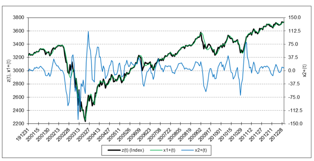
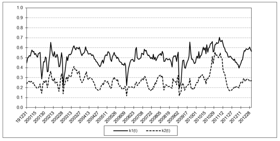
For the three charts above:
The results are hypothetical results and are NOT an indicator of future results and do NOT represent returns that any investor actually attained. Indexes are unmanaged, do not reflect management or trading fees, and one cannot invest directly in an index.

Bloomberg U.S. Aggregate Bond Index

For the three charts above:
The results are hypothetical results and are NOT an indicator of future results and do NOT represent returns that any investor actually attained. Indexes are unmanaged, do not reflect management or trading fees, and one cannot invest directly in an index.

Euro

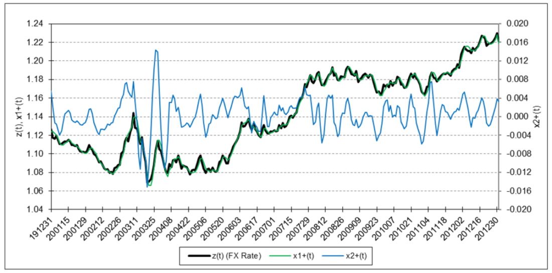
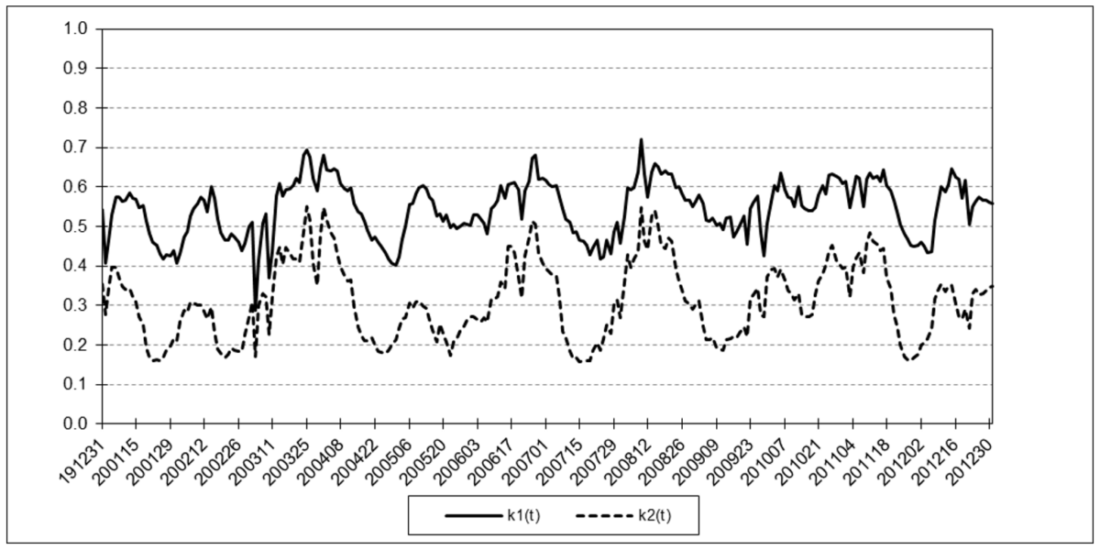
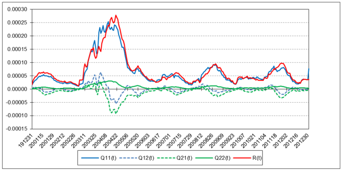
For the three charts above:
The results are hypothetical results and are NOT an indicator of future results and do NOT represent returns that any investor actually attained. Indexes are unmanaged, do not reflect management or trading fees, and one cannot invest directly in an index.

Notes:

• The filter equations in Appendix 1 are shown in non-matrix form for clarity.
• Because the measurement noise variance R(t) and process noise covariance Q(t) may in actual practice become negative definite when performing the estimate calculations, the absolute values of the summation terms of R(t), Q₁₁(t), and Q₂₂(t) are used ⁽⁶⁾.
• In order to minimize potential problems in the initialization process, an expanding time window, i.e., including noise samples at time steps 1 to t, is used to calculate the process noise and measurement noise mean and covariance estimates for time steps 1 through N-1, after which the sliding time window of length N is used.
• In order to minimize potential roundoff errors, the Joseph stabilized form of the state estimate covariance measurement update P⁺(t) equations is used.

References

1. Kalman, R. E., “A New Approach to Linear Filtering and Prediction Problems”, Journal of Basic Engineering, 82 (1), 35-45, March 1960.

2. 6. Myers, K. A. and Tapley, B. D., “Adaptive Sequential Estimation with Unknown Noise Statistics”, IEEE Transactions on Automatic Control, AC-21 (4), 520-523, August 1976.

3. Stengel, R. F., Optimal Control and Estimation, Dover Publications, Inc., 1994.

4. Lopez de Prado, M. and Rebonato, R., “Kinetic Component Analysis”, Journal of Investing, 25 (3), 142-154, Fall 2016.

5. Kalata, P. R., “The Tracking Index: A Generalized Parameter for α-β and α-β-γ Target Trackers”, IEEE Transactions on Aerospace and Electronic Systems, AES-20 (2), 174-182, March 1984.