A Vector Autoregression Trading Model

Excerpt

The vector autoregression (VAR) framework is common in econometrics for modelling correlated variables with bi-directional relationships and feedback loops. If you google “vector autoregression” you’ll find all sorts of academic papers related to modelling the effects of monetary and fiscal policy on various aspects of the economy. This is only of passing interest to traders.

However, if we consider that the VAR framework finds application in the modelling of correlated time series, the implication being that correlation implies a level of forecasting utility, then perhaps we could model a group of related financial instruments and make predictions that we can translate into trading decisions?

So we’ll give that a try. But first, a brief overview of VAR models.

Overview of VAR models

The univariate autoregression (AR) is a model of a time series as a function of past values of itself:

Yt=α+β1Yt−1+β2Yt−2

That’s an AR(2) model because it uses two previous values in the time series Y to estimate the next value. The name of the game is figuring out how many previous values to use, and estimating the coefficients (the β s) and the intercept (α ).

A vector autoregression (VAR) is an extension of this idea. It models multiple time series that affect one another together, as a system. It specifically allows for bi-directional relationships such as feedback loops, where say an increase in variable X may predict an increase in variable Y , but equally an increase in variable Y may predict an increase in variable X .

Here’s a VAR(1) model of two time series, Y1 and Y2 :

Y1,t=α1+β11,1Y1,t−1+β12,1Y2,t−1+ϵ1,t
Y2,t=α2+β21,1Y1,t−1+β22,1Y2,t−1+ϵ2,t

The model uses a single lag of each time series to predict the next values of both time series. It requires the estimation of four coefficients and two intercepts.

Just looking at the single lag case, you get a sense that these models have lots of parameters. Which of course triggers all the usual alarm bells around overfitting. In fact, if we have N time series and p lags in a VAR model, we must estimate N+Np2 parameters!

How do you figure out the number of lags?

Standard practice in econometrics is to use an information criterion. It’s questionable how useful that would be in modelling financial asset returns, and in my view it makes sense to stick with a single lag unless you have a compelling reason to do otherwise.

If you must, lean towards the Bayesian information criterion (BIC), which introduces a penalty term for the number of parameters in the model (the Aikake information criterion does too, but the BIC’s penalty is bigger).

---

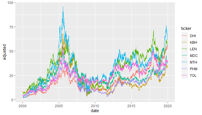
In this example, our group of stocks appeared in the network model of stock relationships that we built using the Graphical Lasso. This is only a single input into the universe selection model that we trade with, but it will do fine for demonstrating this VAR model. We’ll take the stocks in the little purple cluster consisting of residential construction stocks:

# Extract basket prices
tickers <- c('KBH', 'LEN', 'PHM', 'DHI', 'TOL', 'MTH', 'MDC')

This group is a fairly arbitrary choice – the basket is small enough that we can explore VAR models efficiently but other than that there’s nothing particularly special about it. Other than the fact that the Graphical Lasso identified relationships among the group’s stocks.

You can get historical prices and volumes for these tickers via tidyquant::tq_get, which wraps quantmod::getSymbols:

### VAR MODEL STRATEGY ###

library(tidyquant)
library(tidyverse)


# Load basket prices
tickers <- c('KBH', 'LEN', 'PHM', 'DHI', 'TOL', 'MTH', 'MDC')
basket_prices <- tq_get(tickers, get='stock.prices', from='2000-01-01', to = '2020-01-01') %>%
rename(ticker = symbol)

basket_prices %>%
ggplot(aes(x = date, y = adjusted)) +
geom_line(aes(color = ticker))

Plotting the price series:

Visit Robot Wealth website to download the code and read the full article:
https://robotwealth.com/a-vector-autoregression-trading-model/