Volatility And Measures Of Risk-Adjusted Return With Python

Volatility is an important factor to consider for traders since volatility can greatly impact the returns of an investment. A volatile stock or the market can be taken care of with the help of measures to adjust the risk.

In this post, we will see how to compute historical volatility in Python and the different measures of risk-adjusted return based on it.

This blog covers:

• What is meant by volatility?
• Historical volatility
• What is a risk-adjusted return in trading?
• Purpose of risk-adjustment
• Risk-adjusted return ratios in python
• Pros of using the risk-adjusted return ratios
• Cons of using the risk-adjusted return ratios

---

What is meant by volatility?

The upward and downward movement of a security over a period is called volatility. Volatility is one of the factors that define the risk of security. In general, the higher the volatility, the riskier the security. If the price of a security fluctuates slowly over a longer span of time, it is considered to be less volatile.

Conversely, If the price of a security fluctuates rapidly over a small span of time, it is considered to be more volatile. Volatility is measured best by calculating the standard deviation of the annualised returns over a period of time.

Volatility measures the dispersion of returns for given security. It plays a key role in options trading.

The main two volatilities are-

• Implied volatility and
• Historical volatility.

Implied volatility

Let us first talk about implied volatility. Implied volatility is the expected future volatility of the stock. Implied volatility shows the stock’s potential movement, but it doesn’t forecast the direction of the move. If the implied volatility is high, then it means that the market has priced in the potential for large price movements in either direction for the stock.

If the implied volatility is low, the price won’t move as much or may not make any unpredictable changes.

Implied volatility is one of the important deciding factors in the pricing of options. As implied volatility increases, the value of options will increase. That is because an increase in implied volatility suggests an increased range of potential movement for the stock.

The implied volatility is derived from the Black-Scholes formula by entering all the parameters needed to solve for the options price through the Black-Scholes Model and then taking the actual market price of the option and solving back for the implied volatility parameter.

Historical volatility

We will discuss historical volatility here since historical data can best determine a strategy’s performance based on past data.

Historical volatility is derived from time series of past price data, whereas implied volatility is derived using the market price of a traded derivative instrument like an options contract.

Let us see an example by computing the historical volatility of risk-adjusted return for NIFTY.

First, we use the log function from NumPy to compute the logarithmic returns using the NIFTY closing price. Then we use the rolling_std function from Pandas plus the NumPy square root function to calculate the annualised volatility.

The rolling function uses a window of 252 trading days. Each day in the selected lookback period is assigned an equal weight. The user can choose a longer or a shorter period as per his need.

## Computing Volatility
# Load the required modules and packages
import numpy as np
import pandas as pd
import yfinance as yf

# Pull NIFTY data from Yahoo finance
NIFTY = yf.download('^NSEI',start='2018-6-1', end='2022-6-1')

# Compute the logarithmic returns using the Closing price
NIFTY['Log_Ret'] = np.log(NIFTY['Close'] / NIFTY['Close'].shift(1))

# Compute Volatility using the pandas rolling standard deviation function
NIFTY['Volatility'] = NIFTY['Log_Ret'].rolling(window=252).std() * np.sqrt(252)
print(NIFTY.tail(15))

# Plot the NIFTY Price series and the Volatility
NIFTY[['Close', 'Volatility']].plot(subplots=True, color='blue',figsize=(8, 6))

Historical_Volatility.py hosted with ❤ by GitHub

Output:

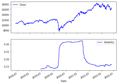
Source: NIFTY data from Yahoo finance

The output above shows that the volatility was the highest between 2020-07 and 2021-06.

---

What is a risk-adjusted return in trading?

Risk-adjusted return is a calculation of the return (or potential return) on the trading of a financial instrument such as a stock. Risk-adjusted returns are often represented as a ratio.

---

Purpose of risk-adjustment

Risk-adjusted return is a critical element to successful long-term investing and the one often overlooked and usually misunderstood by traders new in the field. Risk-adjusted returns are perhaps the most important yet least understood part of investing.

It is always better to weigh the return potential of any investment against the risks it takes so that the risk-return ratio is well understood before making the investment decision.

---

Risk-adjusted return ratios in python

Let us now find out the various measures along with the formula of each for risk-adjusted return in Python. The following are the measures:

• Sharpe ratio
• Information ratio
• Modigliani ratio (M2 ratio)
• Treynor Ratio
• Jensen’s Alpha
• R-squared
• Sortino Ratio

​​Sharpe ratio

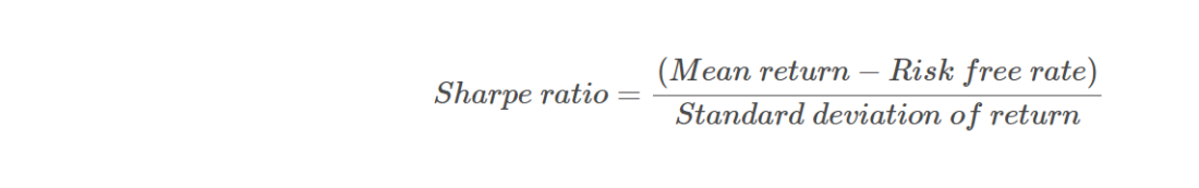
The Sharpe ratio introduced in 1966 by Nobel laureate William F. Sharpe is a measure for calculating risk-adjusted return. The Sharpe ratio is the average return earned in excess of the risk-free rate per unit of volatility.

Here is the formula for Sharpe ratio:

Following is the code to compute the Sharpe ratio in python.

# Sharpe Ratio function
def sharpe(returns, daily_risk_free_rate, days=252):
volatility = returns.std()
sharpe_ratio = (returns.mean() - daily_risk_free_rate) / volatility * np.sqrt(days)
return sharpe_ratio

Sharpe_Ratio.py hosted with ❤ by GitHub

Information ratio (IR)

The information ratio is an extension of the Sharpe ratio which adds the returns of a benchmark portfolio to the inputs. It measures a trader’s ability to generate excess returns relative to a benchmark.

Formula for Information ratio is as follows:

The “tracking error” mentioned above in the formula is the standard deviation of the excess return with respect to the benchmark rate of return.

Following is the code to compute the Information ratio in python.

# Information Ratio
import numpy as np
def information_ratio(returns, benchmark_returns, days=252):
return_difference = returns - benchmark_returns
volatility = return_difference.std()
information_ratio = return_difference.mean() / volatility * np.sqrt(days)
return information_ratio

Information_Ratio.py hosted with ❤ by GitHub

Modigliani ratio (M2 ratio)

The Modigliani ratio measures the returns of the portfolio, adjusted for the risk of the portfolio relative to that of some benchmark.

To calculate the M2 ratio, we first calculate the Sharpe ratio and then multiply it by the annualised standard deviation of a chosen benchmark. We then add the risk-free rate to the derived value to give an M2 ratio.

The Modigliani ratio goes as follows:

Following is the code to compute the Modigliani ratio in python.

# Modigliani Ratio
import numpy as np
def modigliani_ratio(returns, benchmark_returns, rf, days=252):
volatility = returns.std()
sharpe_ratio = (returns.mean() - rf) / volatility * np.sqrt(days)
benchmark_volatility = benchmark_returns.std() * np.sqrt(days)
m2_ratio = (sharpe_ratio * benchmark_volatility) + rf
return m2_ratio

Modigliani_Ratio.py hosted with ❤ by GitHub

Treynor ratio

The Treynor ratio was developed by Jack Treynor, an American economist who was one of the inventors of the Capital Asset Pricing Model (CAPM).

The Treynor ratio is a risk/return measure that allows traders to adjust a portfolio’s returns for systematic risk. A higher Treynor ratio result means a portfolio with the probability of higher returns.

The formula for the Treynor Ratio is:

Following is the python code for the Treynor ratio.

import numpy as np
import pandas as pd

def cumulative_returns(df):
return (df[-1]/df[0])-1

def Treynor_Ratio(pv,ticker_name,start,end,shares,cash,rf=0):
tickers = [ticker_name]
ticker_name_adj_close = get_adjusted_close(tickers,start,end)
ticker_name_pv = Portfolio_Value(comp_adj_close,shares,cash)
ticker_name_returns = daily_returns(comp_pv)
port_returns = daily_returns(pv)
covariance = np.cov(port_returns,ticker_name_returns)[0][1]
variance = np.var(ticker_name_returns)
beta = covariance/variance
Treynor_Ratio = (cumulative_returns(pv) - rf)/beta

Treynor_ratio.py hosted with ❤ by GitHub

Jensen’s alpha

The Jensen’s alpha, is a risk-adjusted performance measure that represents the average return on a portfolio or investment, above or below that predicted by the capital asset pricing model (CAPM).

Given are the portfolio’s or investment’s beta and the average market return.

The formula for Jensen’s alpha is:

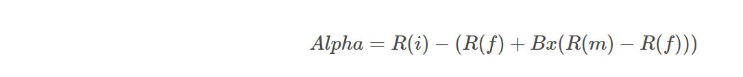
where,

R(i) = the realized return of the portfolio or investment

R(m) = the realized return of the appropriate market index

R(f) = Risk free rate

B = the beta of the portfolio of investment with respect to the chosen market index

In python, we will calculate Jensen’s alpha as follows:

import numpy as np
import pandas as pd
import statsmodels.regression.linear_model as lm
import statsmodels.tools.tools as ct

# Jensen’s alpha’s performance metric data
returns = pd.read_csv(‘Data_file_link’, index_col=’Date’, parse_dates=True)

# Jensen’s alpha’s performance metric calculation
returns.loc[:CT’] = ct.add_constant(returns)

# Using risk free rate of ticker and risk free rate of market for calculating Jensen’s alpha
alphaj = lm.OLS(returns[‘TICKER-RF’], returns[[‘CT’,  ‘MKT-RF’]], hasconst=bool).fit()
print (‘Jensen Alpha Linear Regression Summary’)
print(alphaj.summary())

Jensen_alpha.py hosted with ❤ by GitHub

R-squared

The R squared is the proportion of the variation in the dependent variable that is predictable from the independent variable(s).

It is a statistical ratio whose main purpose is either the prediction of future outcomes or the testing of hypotheses, on the basis of the related information. It provides a measure of how well-observed outcomes are replicated by the model, based on the proportion of total variation of outcomes explained by the model.

The formula for R-squared is as follows:

Let us see how R-squared can be calculated using Python and here is the code for the same:

from sklearn.linear_model import LinearRegression

# initiate linear regression model
model = LinearRegression()

# define predictor and response variables
X, y = df[["variable_1", "variable_2"]], df.result

# fit regression model
model.fit(X, y)

# calculate R-squared of regression model
r_squared = model.result(X, y)

# view R-squared value
print(r_squared)

R_squared.py hosted with ❤ by GitHub

Sortino ratio

The Sortino ratio is similar to Sharpe ratio, except the Sharpe ratio involves both upward and downward volatility while the Sortino ratio represents only downward volatility.

Just like the Sharpe ratio, the higher the Sortino ratio, the better the return for unit risk.

Since most investors are only concerned about the downward volatility, the Sortino ratio represents a more realistic picture of the downward risk.

The choice of using the Sortino or Sharpe ratio for evaluating an investment is solely based on the individual, whether he/she wants to analyze the total volatility or the downside volatility. Both are commonly used for different applications.

Sortino ratio is given by the equation:

Let us now see how to calculate the Sortino ratio in python. Here is the python code for the same:

# Sortino Ratio function

def sortino(returns, daily_risk_free_rate, days=252):
volatility = returns.std()
sortino_ratio = (expected_returns - daily_risk_free_rate) / volatility * np.sqrt(days)
return sortino_ratio

Sortino_Ratio.py hosted with ❤ by GitHub

Thus, this is how we compute historical volatility in python, and we also went through the different measures of risk-adjusted return based on it.

You can learn to optimise your portfolio in Python using Monte Carlo Simulation.

Visit QuantInsti to read Pros and Cons of using the risk-adjusted return ratios: https://blog.quantinsti.com/volatility-and-measures-of-risk-adjusted-return-based-on-volatility/.