Yield to Maturity and Reinvestment Risk Using R Code

This post shows how the reinvestment risk affects the holding period return of coupon bond using R code.

Introduction

At first, we need to make a distinction between par yield and YTM (Yield to Maturity).

Par Yield

The par yield is the coupon rate of a par bond at an issuance. A par bond has a price such as 1 or 100 or 100000 which is the principal amount. Hence, the discount rate which make this bond price to a par is also par yield. It is important that the par yield is defined only with an issuance assumption.

YTM (Yield to Maturity)

YTM is the annualized rate of return (internal rate of return; IRR) that makes a bond price to the current market price. From this definition, YTM is interpreted as the expected yield when holding bond to maturity.

But there are two assumptions regarding YTM as follows.

1. Roll rate (interest rate applied to cash flows received) is equal to YTM.
2. YTM at issuance assumption (par yield) is equal to the coupon rate when timing of interest payment is in arrears not in advance.

Hence, every time when coupon payment is made, this cash flow is required to be reinvested at the same rate of YTM.

Also, if interest payments are made in advance, YTM is higher than coupon rate of the standard coupon bond with in arrears interest payments because compounding period for reinvestment is one interest conversion period such as one quarter longer than otherwise.

As we assume a par bond at issuance, let YTM₀ denote a par yield and YTM_t denote YTM at time t (pricing date).

Reinvestment Risk

When we hold a coupon bond to maturity, can we always obtain YTM₀ as the holding period return? No, it is not always. It is only attainable when all YTM_t is equal to the YTM₀. Reinvestment risk happens when these two YTMs are different.

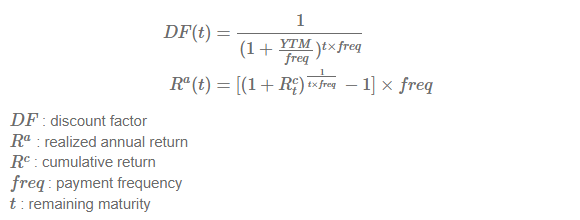
Discount Factor and Realized Return

Sample Cash Flow Schedule for Coupon Bond

Now let’s look at examples. As a sample trade, consider the following 3-maturity semi-annual coupon bond with coupon rate of 4% and notional amount of 100. The following table demonstrates a row-wise stream of coupon and principal payments and column-wise time passages.

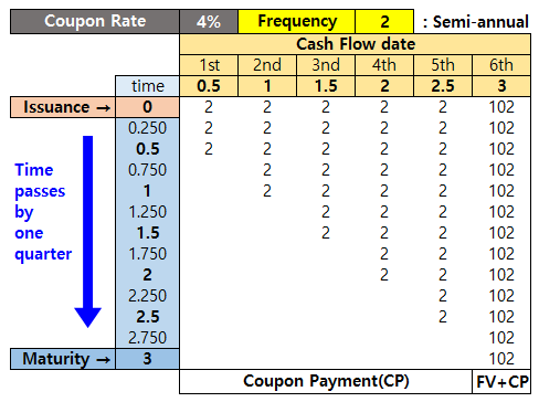
From the above table, time = 0 is the date when you issue or buy a bond. When you make an issuance, par yield (YTM₀) is equal to coupon rate. In the following example, we consider the case of new issuance at time 0. But the logic behind this also holds true for the case of buying at time 0.

For illustration purpose, we use Excel calculation. In the following four cases, green lower triangular part indicates the reinvestment process. After cash flow is received, this amount is reinvested at YTM_t  which may be equal to or different with YTM₀. It depends on market environment.

Quarterly returns and cumulative returns are calculated using both the present values of future cash flows and compounded values of past cash flows received.

1) No compounding : YTM_t>0 = 0

Before discussing the reinvestment risk, let’s see the case of no compounding. This case will makes our understanding of reinvestment process more clear.

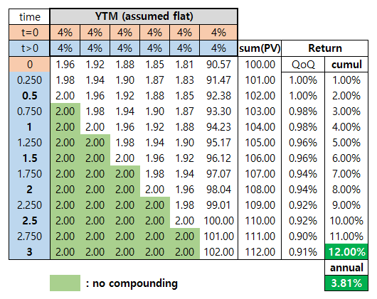
In this no compounding case, interest payments made at earlier times are not reinvested (roll rate is zero) and stay 2($) until maturity. Since any proceeds are not generated from cash flows received, realized annual return is 3.81% which is less than YTM₀.

2) YTM_t>0 = YTM₀

When reinvestment risk is absent, in other words, roll rate is equal to YTM₀, holding period return until maturity is YTM₀ as follows.

In this case, interest payment made at earlier times are reinvested at 4% roll rate until maturity. Since additional return of reinvestment is generated, realized annual return is 4% which is the same value as the YTM₀.

3) YTM_t>0 > YTM₀

When roll rate is higher than YTM₀, holding period return until maturity is also higher than YTM₀ as follows.

In this case, interest payment made at earlier times are reinvested at 6% roll rate until maturity. Realized annual return is 4.1% which is higher than the YTM₀. This means that when bond strategy is the buy-and-hold and market interest rate increases, the cash flows received are reinvested in higher yield.

4) YTM_t>0 < YTM₀

When roll rate is lower than YTM₀, holding period return until maturity is also lower than YTM₀ as follows.

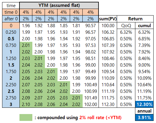
In this case, interest payment made at earlier times are reinvested at 2% roll rate until maturity. Realized annual return is 3.9% which is lower than the YTM₀. This means that when bond strategy is the buy-and-hold and market interest rate decreases, the cash flows received are reinvested in lower yield.

In conclusion, buy-and-hold strategy guarantees fixed payments of coupons and principal amount but earlier received coupon payments are exposed to interest rate risk. This is called the reinvestment risk.

R code for Reinvestment Risk

The following R code demonstrates the calculation of discounted cash flows from coupon bond at every quarterly pricing time t. Besides quarterly price of bonds, This code also shows the reinvestment process of cash flows received at every quarter.

#=========================================================================#
# Financial Econometrics & Derivatives, ML/DL using R, Python, Tensorflow  
# by Sang-Heon Lee 
#
# https://shleeai.blogspot.com
#-------------------------------------------------------------------------#
# Demonstrate Reinvestment Risk with YTM and varying roll rate
#=========================================================================#
 
graphics.off()      # clear all graphs
rm(list = ls())     # remove all files from your workspace
    
iss_maty = 3        # issuance maturity in year
freq     = 2        # semi-annual coupon payment
face_val = 100      # face value
cpn_rate = 0.04     # coupon rate
dt       = 0.25     # time interval
nall     = freq*iss_maty
 
# cash flow table
df.cf <- data.frame(no   = integer(nall), 
                    date = double (nall), 
                    amt  = double (nall))
 
for(i in 1:nall) {
    
    df.cf$no  [i] <- i
    df.cf$date[i] <- i/freq
    df.cf$amt [i] <- (cpn_rate/freq)*face_val
    if(i==freq*iss_maty) df.cf$amt[i] <- df.cf$amt[i] + face_val
}
df.cf
 
# time line
v.time <- seq(0,iss_maty,dt)
 
#------------------------------------------------
# YTM pricing and Reinvestment Risk
#------------------------------------------------
 
    # YTM for t > 0
    ytm_after_0= 0.04  # 1) roll rate (4%) = 4%
    #ytm_after_0= 0.06  # 2) roll rate (6%) > 4%
    #ytm_after_0 = 0.02  # 3) roll rate (2%) < 4%
 
    # table for time line and cash flow schedule
    df.bond <- data.frame()
 
    for(t in v.time) { # As time t elapsed
 
        # use df.cf temporarily
        df <- df.cf
        
        # YTM (t>0) for discounting
        # t = 0 : par yield  (make price to a par)
        # t > 0 : yield to maturity (market yield) 
        rate = ifelse(t==0, cpn_rate, ytm_after_0)
 
        # discount factor
        df$DF = 1/(1+rate/freq)^((df$date-t)*freq)
        
        # present value of cash flow
        df$PV = df$amt*df$DF
        
        # add rows to df.bond with sum(PV) = price
        df.bond <- rbind(df.bond, c(df$PV, sum(df$PV)))
    }
 
    # append time to the left
    df.bond <- cbind(v.time, df.bond)
    
    # set column names for convenience
    colnames(df.bond) <- c("time", paste0("cf",1:nall), "price")
    
    # quarter on quarter (qoq) returns 
    nr <- nrow(df.bond)
    df.bond$qoq_rtn <- c(0,df.bond$price[2:nr]/
                           df.bond$price[1:(nr-1)] - 1)
    
    # cumulative returns
    df.bond$cum_rtn <- 0
    for(i in 2:nr) { 
        df.bond$cum_rtn[i] <- (1+df.bond$cum_rtn[i-1])*
                              (1+df.bond$qoq_rtn[i])-1
    }
 
    # 3-year returns
    print(paste0("3-year return = ", 
                 round(100*((1+df.bond$cum_rtn[nr])^(1/nall)-1)*freq,4),
                 "% when roll rate is ", 100*ytm_after_0, 
                 "% and YTM at time 0 is ", 100*cpn_rate,"%"))
 
    # rounding for printing out
    df.bond[,2:8] <- round(df.bond[,2:8],2)
    df.bond$qoq_rtn <- round(df.bond$qoq_rtn,5)
    df.bond$cum_rtn <- round(df.bond$cum_rtn,3)
    df.bond

By changing “ytm_after_0” variable in R code, three types of result are obtained. We can easily find that these results are consistent with the above Excel counterparts respectively.

Firstly, under the condition that roll rate is the same as YTM₀, the following result can be obtained.

[1] "3-year return = 4% when roll rate is 4% and YTM at time 0 is 4%"
> 
   time  cf1  cf2  cf3  cf4  cf5    cf6  price qoq_rtn cum_rtn
1  0.00 1.96 1.92 1.88 1.85 1.81  90.57 100.00 0.00000   0.000
2  0.25 1.98 1.94 1.90 1.87 1.83  91.47 101.00 0.00995   0.010
3  0.50 2.00 1.96 1.92 1.88 1.85  92.38 102.00 0.00995   0.020
4  0.75 2.02 1.98 1.94 1.90 1.87  93.30 103.01 0.00995   0.030
5  1.00 2.04 2.00 1.96 1.92 1.88  94.23 104.04 0.00995   0.040
6  1.25 2.06 2.02 1.98 1.94 1.90  95.17 105.08 0.00995   0.051
7  1.50 2.08 2.04 2.00 1.96 1.92  96.12 106.12 0.00995   0.061
8  1.75 2.10 2.06 2.02 1.98 1.94  97.07 107.18 0.00995   0.072
9  2.00 2.12 2.08 2.04 2.00 1.96  98.04 108.24 0.00995   0.082
10 2.25 2.14 2.10 2.06 2.02 1.98  99.01 109.32 0.00995   0.093
11 2.50 2.16 2.12 2.08 2.04 2.00 100.00 110.41 0.00995   0.104
12 2.75 2.19 2.14 2.10 2.06 2.02 101.00 111.51 0.00995   0.115
13 3.00 2.21 2.16 2.12 2.08 2.04 102.00 112.62 0.00995   0.126

Secondly, under the condition that roll rate is higher than YTM₀, the following result can be generated.

[1] "3-year return = 4.0967% when roll rate is 6% and YTM at time 0 is 4%"
> 
   time  cf1  cf2  cf3  cf4  cf5    cf6  price  qoq_rtn cum_rtn
1  0.00 1.96 1.92 1.88 1.85 1.81  90.57 100.00  0.00000   0.000
2  0.25 1.97 1.91 1.86 1.80 1.75  86.70  95.99 -0.04009  -0.040
3  0.50 2.00 1.94 1.89 1.83 1.78  87.99  97.42  0.01489  -0.026
4  0.75 2.03 1.97 1.91 1.86 1.80  89.30  98.87  0.01489  -0.011
5  1.00 2.06 2.00 1.94 1.89 1.83  90.63 100.34  0.01489   0.003
6  1.25 2.09 2.03 1.97 1.91 1.86  91.98 101.84  0.01489   0.018
7  1.50 2.12 2.06 2.00 1.94 1.89  93.34 103.35  0.01489   0.034
8  1.75 2.15 2.09 2.03 1.97 1.91  94.73 104.89  0.01489   0.049
9  2.00 2.19 2.12 2.06 2.00 1.94  96.14 106.45  0.01489   0.065
10 2.25 2.22 2.15 2.09 2.03 1.97  97.58 108.04  0.01489   0.080
11 2.50 2.25 2.19 2.12 2.06 2.00  99.03 109.65  0.01489   0.096
12 2.75 2.28 2.22 2.15 2.09 2.03 100.50 111.28  0.01489   0.113
13 3.00 2.32 2.25 2.19 2.12 2.06 102.00 112.94  0.01489   0.129

Thirdly, under the condition that roll rate is lower than YTM₀, the following result can be returned.

[1] "3-year return = 3.9056% when roll rate is 2% and YTM at time 0 is 4%"
> 
   time  cf1  cf2  cf3  cf4  cf5    cf6  price qoq_rtn cum_rtn
1  0.00 1.96 1.92 1.88 1.85 1.81  90.57 100.00 0.00000   0.000
2  0.25 1.99 1.97 1.95 1.93 1.91  96.57 106.32 0.06323   0.063
3  0.50 2.00 1.98 1.96 1.94 1.92  97.05 106.85 0.00499   0.069
4  0.75 2.01 1.99 1.97 1.95 1.93  97.53 107.39 0.00499   0.074
5  1.00 2.02 2.00 1.98 1.96 1.94  98.02 107.92 0.00499   0.079
6  1.25 2.03 2.01 1.99 1.97 1.95  98.51 108.46 0.00499   0.085
7  1.50 2.04 2.02 2.00 1.98 1.96  99.00 109.00 0.00499   0.090
8  1.75 2.05 2.03 2.01 1.99 1.97  99.49 109.54 0.00499   0.095
9  2.00 2.06 2.04 2.02 2.00 1.98  99.99 110.09 0.00499   0.101
10 2.25 2.07 2.05 2.03 2.01 1.99 100.49 110.64 0.00499   0.106
11 2.50 2.08 2.06 2.04 2.02 2.00 100.99 111.19 0.00499   0.112
12 2.75 2.09 2.07 2.05 2.03 2.01 101.49 111.75 0.00499   0.117
13 3.00 2.10 2.08 2.06 2.04 2.02 102.00 112.30 0.00499   0.123

From this post, we can learn the reinvestment risk of a coupon bond. It is worth noting that 1) YTM is attainable when a roll rate is the same as YTM and 2) The argument that coupon rate is equal to YTM at issuance (par yield) is only applied to standard coupon bond with in arrears interest payment schedule. Unlike the standard coupon bond, coupon bond with in advance interest payment has a higher YTM than coupon rate at an issuance.

Next time, we will calculate the holding period returns of the benchmark bond portfolio strategies such as bullet, ladder, buy-and-hold, barbell, and so on.

Originally posted on SHLee AI Financial Model.