Forward Propagation In Neural Networks: Components and Applications – Part II

Learn about the forward propagation algorithm with Part I.

Forward propagation vs backward propagation in neural network

Below is the table for a clear difference between forward and backward propagation in the neural network.

Aspect	Forward Propagation	Backward Propagation
Purpose	Compute the output of the neural network given inputs	Adjust the weights of the network to minimise error
Direction	Forward from input to output	Backwards, from output to input
Calculation	Computes the output using current weights and biases	Updates weights and biases using calculated gradients
Information flow	Input data -> Output data	Error signal -> Gradient updates
Steps	1. Input data is fed into the network.2. Data is processed through hidden layers.3. Output is generated.	1. Error is calculated using a loss function.2. Gradients of the loss function are calculated.3. Weights and biases are updated using gradients.
Used in	Prediction and inference	Training the neural network

Next, let us see the forward propagation in different types of neural networks.

---

Forward propagation in different types of neural networks

Forward propagation is a key process in various types of neural networks, each with its own architecture and specific steps involved in moving input data through the network to produce an output.

Forward propagation is a fundamental process in various types of neural networks, including:

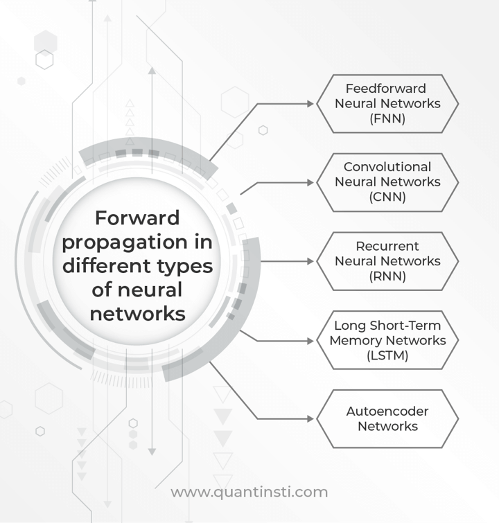
• Feedforward Neural Networks (FNN): In FNNs, also known as Multi-layer Perceptrons (MLPs), forward propagation involves passing the input data through the network’s layers from the input layer to the output layer without any feedback loop.
• Convolutional Neural Networks (CNN): In CNNs, forward propagation involves passing the input data through convolutional layers, pooling layers, and fully connected layers. Convolutional layers apply convolution operations to the input data, extracting features. Pooling layers reduce the spatial dimensions of the data. Fully connected layers perform the final classification.
• Recurrent Neural Networks (RNN): In RNNs, forward propagation involves passing the input sequence through the network’s layers. RNNs have recurrent connections, allowing information to persist. Each step in the sequence feeds the output of the previous step back into the network.
• Long Short-Term Memory Networks (LSTM): LSTM networks are a type of RNN designed to address the vanishing gradient problem. Forward propagation in LSTMs involves passing input sequences through gates that control the flow of information. These gates include input, forget, and output gates, which regulate the flow of information in and out of the cell.
• Autoencoder Networks: In autoencoder networks, forward propagation involves encoding the input data into a lower-dimensional representation and then decoding it back to the original input space.

Moving forward, let us discuss the components of forward propagation.

---

Components of forward propagation

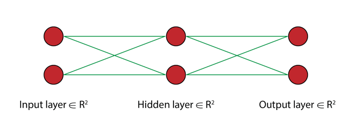
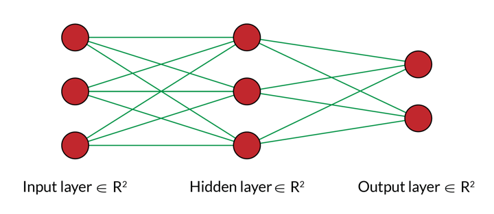
In the above diagram, we see a neural network consisting of three layers. The first and the third layer are straightforward, input and output layers. But what is this middle layer and why is it called the hidden layer?

Now, in our example, we had just one equation, thus we have only one neuron in each layer.

Nevertheless, the hidden layer consists of two functions:

• Pre-activation function: The weighted sum of the inputs is calculated in this function.
• Activation function: Here, based on the weighted sum, an activation function is applied to make the network non-linear and make it learn as the computation progresses. The activation function uses bias to make it non-linear.

Going forward, we must check out the applications of forward propagation to learn about the same in detail.

---

Applications of forward propagation

In this example, we will be using a 3-layer network (with 2 input units, 2 hidden layer units, and 2 output units). The network and parameters (or weights) can be represented as follows.

Let us say that we want to train this neural network to predict whether the market will go up or down. For this, we assign two classes Class 0 and Class 1.

Here, Class 0 indicates the data point where the market closes down, and conversely, Class 1 indicates that the market closes up. To make this prediction, a train data(X) consisting of two features x1, and x2. Here x1 represents the correlation between the close prices and the 10-day simple moving average (SMA) of close prices, and x2 refers to the difference between the close price and the 10-day SMA.

In the example below, the data point belongs to class 1. The mathematical representation of the input data is as follows:

X = [x1, x2] = [0.85,.25] y= [1]

Example with two data points:

The output of the model is categorical or a discrete number. We need to convert this output data into a matrix form. This enables the model to predict the probability of a data point belonging to different classes. When we make this matrix conversion, the columns represent the classes to which that example belongs, and the rows represent each of the input examples.

In the matrix y, the first column represents class 0 and second column represents class 1. Since our example belongs to Class 1, we have 1 in the second column and zero in the first.

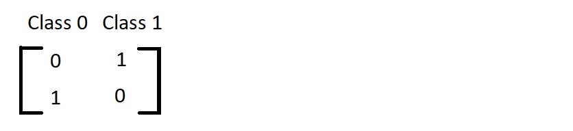
This process of converting discrete/categorical classes to logical vectors/matrices is called One-Hot Encoding. It’s sort of like converting the decimal system (1,2,3,4….9) to binary (0,1,01,10,11). We use one-hot encoding as the neural network cannot operate on label data directly. They require all input variables and output variables to be numeric.

In neural network learning, apart from the input variable, we add a bias term to every layer other than the output layer. This bias term is a constant, mostly initialised to 1. The bias enables moving the activation threshold along the x-axis.

When the bias is negative the movement is made to the right side, and when the bias is positive the movement is made to the left side. So a biassed neuron should be capable of learning even such input vectors that an unbiased neuron is not able to learn. In the dataset X, to introduce this bias we add a new column denoted by ones, as shown below.

Let us randomly initialise the weights or parameters for each of the neurons in the first layer. As you can see in the diagram we have a line connecting each of the cells in the first layer to the two neurons in the second layer. This gives us a total of 6 weights to be initialized, 3 for each neuron in the hidden layer. We represent these weights as shown below.

Here, Theta₁ is the weights matrix corresponding to the first layer.

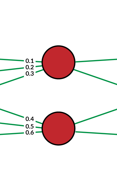
The first row in the above representation shows the weights corresponding to the first neuron in the second layer, and the second row represents the weights corresponding to the second neuron in the second layer. Now, let’s do the first step of the forward propagation, by multiplying the input value for each example by their corresponding weights which are mathematically shown below.

Theta₁ * X

Before we go ahead and multiply, we must remember that when you do matrix multiplications, each element of the product, X*θ, is the dot product sum of the row in the first matrix X with each of the columns of the second matrix θ.

When we multiply the two matrices, X and θ, we are expected to multiply the weights with the corresponding input example values. This means we need to transpose the matrix of example input data, X so that the matrix will multiply each weight with the corresponding input correctly.

Here z² is the output after matrix multiplication, and X_t is the transpose of X.

The matrix multiplication process:

Let us say that we have applied a sigmoid activation after the input layer. Then we have to element-wise apply the sigmoid function to the elements in the z² matrix above. The sigmoid function is given by the following equation:

After the application of the activation function, we are left with a 2×1 matrix as shown below.

Here a⁽²⁾ represents the output of the activation layer.

These outputs of the activation layer act as the inputs for the next or the final layer, which is the output layer. Let us initialize another random weights/parameters called Theta₂ for the hidden layer. Each row in Theta₂ represents the weights corresponding to the two neurons in the output layer.

After initializing the weights (Theta₂), we will repeat the same process that we followed for the input layer. We will add a bias term for the inputs of the previous layer. The a⁽²⁾ matrix looks like this after the addition of bias vectors:

Let us see how the neural network looks like after the addition of the bias unit:

Before we run our matrix multiplication to compute the final output z³, remember that before in z² calculation we had to transpose the input data a¹ to make it “line up” correctly for the matrix multiplication to result in the computations we wanted. Here, our matrices are already lined up the way we want, so there is no need to take the transpose of the a⁽²⁾ matrix. To understand this clearly, ask yourself this question: “Which weights are being multiplied with what inputs?”. Now, let us perform the matrix multiplication:

z³ = Theta₂*a⁽²⁾ where z³ is the output matrix before the application of an activation function.

Here for the last layer, we will be multiplying a 2×3 with a 3×1 matrix, resulting in a 2×1 matrix of output hypotheses. The mathematical computation is shown below:

After this multiplication, before getting the output in the final layer, we apply an element-wise conversion using the sigmoid function on the z² matrix.

a³ = sigmoid(z³)

Where a³ denotes the final output matrix.

The output of a sigmoid function is the probability of the given example belonging to a particular class. In the above representation, the first row represents the probability that the example belonging to Class 0 and the second row represents the probability of Class 1.

That’s all there is to know about forward propagation in Neural networks.

Author: Chainika Thakar (Originally written by Varun Divakar and Rekhit Pachanekar)

Stay tuned for Part III to lean about forward propagation in trading.

Originally posted on QuantInsti.