


Code along Robot Wealth as they present an analysis of the SPY returns process using the QuantConnect research platform.
Excerpt
Example Research With QuantConnect Code
Using the QuantConnect ecosystem in a typical quant workflow.
Note: This code is meant to be used within QuantConnect research environment
# Import dependecies
import numpy as np
import seaborn as sns
import matplotlib.pyplot as plt
plt.style.use(‘ggplot’) #There is a positive correlation between chart pretiness and risk-adjusted returns
plt.rcParams[‘figure.figsize’] = [10, 7]
# QuantBook Analysis Tool
# Load SPY historical data
qb = QuantBook()
spy = qb.AddEquity(“SPY”)
history = qb.History(qb.Securities.Keys, 5000, Resolution.Daily) #5000 days of SPY daily data
# Drop pandas level
history = history.reset_index().drop(‘symbol’,axis=1)
# Calculate SPY returns and fillna
history[‘returns’] = (history[‘close’].pct_change() * 100).fillna(0)
1. Analysing the return distribution
Now that we have SPY daily returns let’s quickly see what we’re dealing with.
history[‘returns’].describe()
count 5000.000000
mean 0.030071
std 1.235997
min -11.638806
25% -0.443536
50% 0.061797
75% 0.573180
max 11.360371
Name: returns, dtype: float64
Let’s look at the extreme values of returns ie max and min
history[history[‘returns’] == min(history[‘returns’])]

history[history[‘returns’] == max(history[‘returns’])]

The recent corona drawdown is the biggest single-day market drop in history, and we have the biggest up move in 2008.
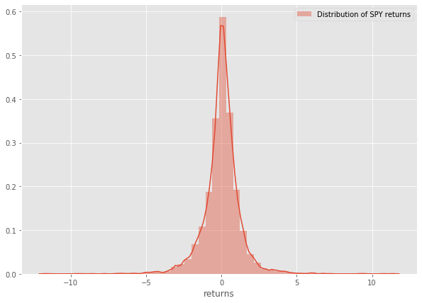
Let’s look at the distribution of daily returns for the SPY
sns.distplot(history[‘returns’],label=’Distribution of SPY returns’) plt.legend()
2. Comparing to a normal distribution
Let’s first create some random data and plot their distribution
random = np.random.normal(scale=1.23,size=500000)
sns.distplot(random,label=’Returns sampled from normal distribution’,color=’blue’)
plt.legend()
random_series = pd.Series(random)
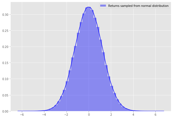
There it is, a beautiful well behaved normal distribution, Let’s see how this compares to our SPY returns distribution.
sns.distplot(history[‘returns’],label=’Distribution of SPY returns’) sns.distplot(random,label=’Returns sampled from normal distribution’) plt.legend()
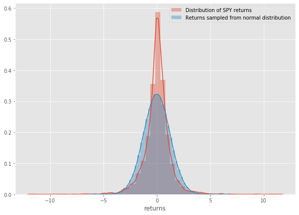
Now the high kurtosis of the SPY returns becomes even more apparent.
So far we’ve learned that:
- SPY returns do resemble random returns
- but they have big tails in their distribution
- which means we can expect outsized moves to the upside and downside, more so than a normal distribution would suggest.
Now let’s look at a simple workflow for researching, seasonal patterns in our financial data.
Visit Robot Wealth to read the next steps Researching possible seasonal patterns and Looking for auto-correlation (trend) in the return process, and to download the sample code: https://robotwealth.com/how-to-be-a-quant-trader-experiments-with-quantconnect/
Disclosure: Interactive Brokers
Information posted on IBKR Campus that is provided by third-parties does NOT constitute a recommendation that you should contract for the services of that third party. Third-party participants who contribute to IBKR Campus are independent of Interactive Brokers and Interactive Brokers does not make any representations or warranties concerning the services offered, their past or future performance, or the accuracy of the information provided by the third party. Past performance is no guarantee of future results.
This material is from Robot Wealth and is being posted with its permission. The views expressed in this material are solely those of the author and/or Robot Wealth and Interactive Brokers is not endorsing or recommending any investment or trading discussed in the material. This material is not and should not be construed as an offer to buy or sell any security. It should not be construed as research or investment advice or a recommendation to buy, sell or hold any security or commodity. This material does not and is not intended to take into account the particular financial conditions, investment objectives or requirements of individual customers. Before acting on this material, you should consider whether it is suitable for your particular circumstances and, as necessary, seek professional advice.