Portfolio Optimisation with MlFinLab: Estimation of Risk

Image Credits: Schwab Intelligent Portfolios™ Asset Allocation White Paper

Risk has always played a very large role in the world of finance with the performance of a large number of investment and trading strategies being dependent on the efficient estimation of underlying market risk. With regards to this, one of the most popular and commonly used representation of risk in finance is through a covariance matrix – higher covariance values mean more volatility in the markets and vice-versa. This also comes with a caveat – empirical covariance values are always measured using historical data and are extremely sensitive to small changes in market conditions. This makes the covariance matrix an unreliable estimator of the true risk and calls for a need to have better estimators.

In this post we will use the RiskEstimators class from MlFinLab which provides several implementations for different ways to calculate and adjust the empirical covariance matrices. Some of these try to remove inherent outliers from the matrix while others focus on removing noise from the empirical values. Throughout this blog post, we will look at a quick description of each algorithm as well as see how we can use the corresponding implementation provided in MlFinLab.

The RiskEstimators class covers seven different algorithms relating to covariance matrix estimators. These algorithms include:

• Minimum Covariance Determinant
• Empirical Covariance
• Covariance Estimator with Shrinkage
• Semi-Covariance Matrix
• Exponentially-Weighted Covariance matrix
• De-Noising Covariance Matrix
• Covariance and Correlation Matrix Transformations

Note: The descriptions of these algorithms are all based upon the descriptions from the scikit-learn User Guide on Covariance Estimation. Infact, most of the methods (except the denoising and detoning ones) in the class are wrappers of sklearn’s covariance methods but with the added functionality of working specifically with financial data e.g. having inbuilt returns calculation.

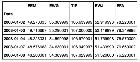
We will import the required libraries and the dataset – a small subset of historical prices of ETFs.

# importing our required libraries
import numpy as np
import pandas as pd
import matplotlib.pyplot as plt
import mlfinlab as ml

# reading in our data
stock_prices = pd.read_csv(‘stock_prices.csv’, parse_dates=True, index_col=’Date’)
stock_prices = stock_prices.dropna(axis=1)

For the purpose of this post, we will only use 5 assets, so the differences between the calculated covariance matrices are easy to see.

stock_prices = stock_prices.iloc[:, :5]
stock_prices.head()

Minimum Covariance Determinant

The Minimum Covariance Determinant (MCD) is a robust estimator of covariance that was introduced by P.J. Rousseeuw. From the scikit-learn User Guide on Covariance Estimation, “the basic idea of the algorithm is to find a set of observations that are not outliers and compute their empirical covariance matrix, which is then rescaled to compensate for the performed selection of observations”. The MlFinLab implementation is a wrap around sklearn’s MinCovDet class, which uses FastMCD algorithm, developed by Rousseeuw and Van Driessen. A detailed description of the algorithm is available in the paper by Mia Hubert and Michiel Debruyne – Minimum Covariance Determinant.

First, we can construct a simple (empirical) covariance matrix for comparison.# A class with function to calculate returns from pricesreturns_estimation = ml.portfolio_optimization.ReturnsEstimators()# Calcualting the data set of returnsstock_returns = returns_estimation.calculate_returns(stock_prices)# Finding the simple covariance matrix from a series of returnscov_matrix = stock_returns.cov()

We can now construct the MCD matrix. One can use minimum_covariance_determinant() method for this purpose.

# A class that has the Minimum Covariance Determinant estimator
risk_estimators = ml.portfolio_optimization.RiskEstimators()

# Finding the Minimum Covariance Determinant estimator on price data and with set random seed to 0
min_cov_det = risk_estimators.minimum_covariance_determinant(stock_prices, price_data=True, random_state=0)

# Transforming our estimation from a np.array to pd.DataFrame
min_cov_det = pd.DataFrame(min_cov_det, index=cov_matrix.index, columns=cov_matrix.columns)

From the above images, you can see that the absolute values in the Minimum Covariance Determinant estimator are lower in comparison to the simple Covariance matrix, which means that the algorithm has eliminated some of the outliers in the data and the resulting covariance matrix estimator is a more robust one. Note that this method achieves the best result when the data has outliers in it.

Maximum Likelihood Covariance Estimator (Empirical Covariance)

Maximum Likelihood Estimator of a sample is an unbiased estimator of the corresponding population’s covariance matrix. This estimation works well when the number of observations is big enough in relation to the number of features.

We can implement this algorithm through the empirical_covariance method() in the MlFinLab library.

# Finding the Empirical Covariance on price data
empirical_cov = risk_estimators.empirical_covariance(stock_prices, price_data=True)

# Transforming Empirical Covariance from np.array to pd.DataFrame
empirical_cov = pd.DataFrame(empirical_cov, index=cov_matrix.index, columns=cov_matrix.columns)

One can observe that the Empirical Covariance is the same as the standard covariance function from the pandas package i.e. the cov()  function.

Visit Hudson and Thames Quantitative Research website to read the full article and download practical code:
https://hudsonthames.org/portfolio-optimisation-with-mlfinlab-estimation-of-risk/