The Graphical Lasso and its Financial Applications

Excerpt

Applying the Graphical Lasso to stock data using R

We’re going to take a universe of US equities and apply the Graphical Lasso algorithm to estimate an inverse covariance matrix. Then, we’ll apply the transform given by the equation above to construct a sparse matrix of partial correlations.

We can think of this sparse matrix as representing a network with edges (connections) between nodes (stocks ) that have some sort of relationship, independent of any of the other variables.

Thinking of our matrix in this way leads us to the concept of a network graph which we can use as a visual tool to aid our understanding of and ability to reason about a large universe of stocks.

Our data consists of daily returns for the top roughly 1,100 US stocks by market cap between 2010 and 2019. Each returns series is standardised to have zero mean and unit variance.

Firstly, we group stocks into clusters based on loadings to statistical factors obtained from Principal Components Analysis (PCA) using the DBSCAN clustering algorithm. In our graph, we will colour stocks according to their cluster. All going well, we should see more connections between stocks within the same cluster.

We’ll gloss over the code for performing the clustering operations here – the subject of another blog post perhaps.

Next, we calculate a covariance matrix of stock returns.

I’ll provide the code for you to reproduce the analysis from this point. We’ll use the glasso package, which implements the Graphical Lasso algorithm, the igraph package, which contains tools for building network graphs, and the threejs and htmlwidgets packages for creating interactive plots.

The first thing we need to do is load these and a few other packages and the data:

# install and load required packages
required.packages <- c('glasso', 'colorRamps', 'igraph', 'RColorBrewer', 'threejs', 'htmlwidgets')
new.packages <- required.packages[!(required.packages %in% installed.packages()[,"Package"])]
if(length(new.packages)) install.packages(new.packages, repos=’http://cran.us.r-project.org’)
library(glasso);library(colorRamps);library(igraph);library(RColorBrewer);library(threejs);library(htmlwidgets);


# load data
load(“./clusters_covmat.RData”)

This will load the covariance matrix into the variable S and a dataframe of tickers and their corresponding clusters into the variable cl.

Then, to apply the Graphical Lasso, we choose a value for rho, which is the regularisation parameter that controls the degree of sparsity in the resulting inverse covariance matrix. Higher values lead to greater sparsity.

In our application, there is no “correct” value of rho, but it can be tuned for your use case.

For instance, if you wanted to isolate the strongest relationships in your data you would choose a higher value rho. If you were interested in preserving more tenuous connections, perhaps identifying stocks with connections to multiple groups, you’d choose a lower value of rho. Finding a sensible value requires experimentation.

It’s also not a bad idea to check for symmetry in the resulting inverse covariance matrix. Assymmetry can arise due to numerical computation and rounding errors, which can cause problems later depending on what you want to do with the matrix.

# estimate precision matrix using glasso
rho <- 0.75
invcov <- glasso(S, rho=rho)
P <- invcov$wi
colnames(P) <- colnames(S)
rownames(P) <- rownames(S)


# check symmetry
if(!isSymmetric(P)) {
P[lower.tri(P)] = t(P)[lower.tri(P)]
}

Next, we calculate the partial correlation matrix and set the terms on the diagonal to zero – this prevents stocks having connections with themselves in the network graph we’ll be shortly constructing:

# calculate partial correlation matrix
parr.corr <- matrix(nrow=nrow(P), ncol=ncol(P))
for(k in 1:nrow(parr.corr)) {
for(j in 1:ncol(parr.corr)) {
parr.corr[j, k] <- -P[j,k]/sqrt(P[j,j]*P[k,k])
}
}
colnames(parr.corr) <- colnames(P)
rownames(parr.corr) <- colnames(P)
diag(parr.corr) <- 0

Now if you run View(parr.corr) in R Studio, you’ll see a very sparse partial correlation matrix. In fact, only about 6,000 of 1.35 million elements will contain non-zeroes! The non-zero elements represent a connection between two stocks, with the strength of the connection determined by the magnitude of the partial correlation. Here’s a snapshot that gives you an idea of the level of sparsity:

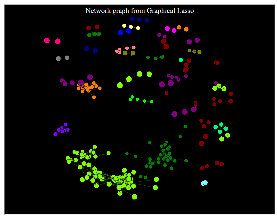
The partial correlation matrix can be used to build a network graph, where stocks are represented as nodes and non-zero elements are represented as edges between two stocks.

The igraph package has some fantastic tools for building, manipulating and displaying graphs. We’ll only use a fraction of the package’s features here, but if you’re interested in getting to know it, check out Katya Ognyanova’s tutorial (it’s really excellent and got me up and running with igraph in a matter of hours).

This next block of code constructs the network graph, assigns a colour to each node according to its cluster and drops any node with no connections.

Visit Robot Wealth website to download the code, and interact the resulting network graph (screenshot below):
https://robotwealth.com/the-graphical-lasso-and-its-financial-applications/