Python: t-SNE Dimensional Reduction Technique

This post shows how to use the t-SNE (t-Distributed Stochastic Neighbor Embedding) in Python, which is a non-linear probabilistic technique for dimensionality reduction.

t-SNE Dimension Reduction

The t-SNE is a nonlinear dimensionality reduction technique used primarily for visualizing high-dimensional data in a lower-dimensional space (often 2D or 3D). It is particularly effective at preserving local relationships between data points while revealing the underlying structure or clusters in the data.

It aims to represent each data point as a two- or three-dimensional point while preserving the similarity between nearby points in the original space.

The t-SNE uses the Kullback-Leibler (KL) divergence to optimize the embedding of high-dimensional data into a lower-dimensional space while preserving the local relationships between data points.

There are numerous valuable resources on Google, such as applications for the MNIST or IRIS datasets with detailed mathematical explanations. Therefore, I won’t reiterate them here. Instead, in this post, I am using different dataset: yield curve data.

In some academic papers, 2-dimensional t-SNE plots of both the original and synthetic data are used to evaluate the quality of data generated by the variational autoencoder (VAE). Generally, higher similarity between these plots indicates better quality

Python Jupyter Notebook Code

Initially, the data preparation process involves downloading the DRA dataset. Empirical yield curve factors are calculated based on the DRA approach. As the scatter plots requires the target value like z value, I use the empirical curvature factor.

import pandas as pd
import numpy as np
import matplotlib.pyplot as plt
from sklearn.manifold import TSNE
 
import requests
from io import StringIO
 
# URL for the data
url = "http://econweb.umd.edu/~webspace/aruoba/research/paper5/DRA%20Data.txt"
 
# Read the data from the URL
response = requests.get(url)
data = StringIO(response.text)
df = pd.read_csv(data, sep="\t", header=0)
 
# Convert yield columns to a matrix divided by 100
df = df.iloc[:, 1:18] / 100
 
# Empiricalyield curve factors
L = df.iloc[:,16]
S = df.iloc[:,0] - df.iloc[:,16]
C = df.iloc[:,8] - df.iloc[:,0] - df.iloc[:,16]
 
# temporary target value
target = C 
 

The following code performs the t-SNE dimension reduction and compares with PCA.

# t-SNE
tsne = TSNE(random_state=42) #, init='pca') #, learning_rate=100)
tsne_results = tsne.fit_transform(df)
tsne1 = pd.DataFrame(tsne_results[:,0])
tsne2 = pd.DataFrame(tsne_results[:,1])
 
# Create a figure with two subplots
fig, axes = plt.subplots(nrows=2, ncols=1, figsize=(6, 8))
 
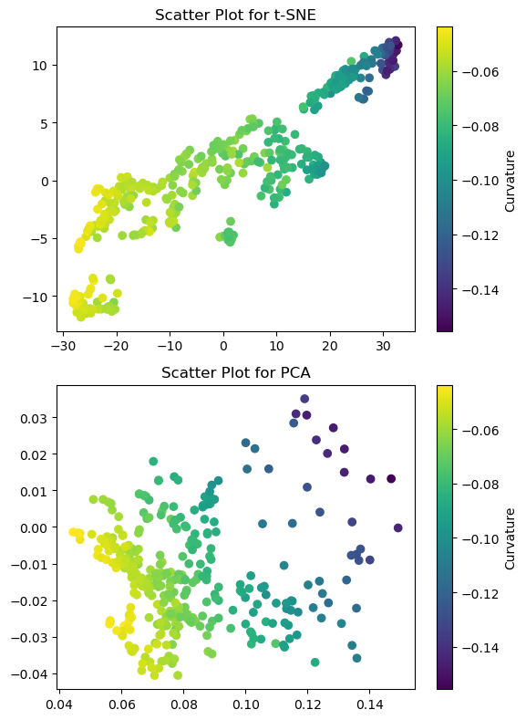
# Scatter plot for t-SNE
sc1 = axes[0].scatter(tsne1, tsne2, c=target)
axes[0].set_title('Scatter Plot for t-SNE')
cbar1 = plt.colorbar(sc1, ax=axes[0])
cbar1.set_label('Curvature')
 
# Scatter plot for yield curve factors
sc2 = axes[1].scatter(L, S, c=target)
axes[1].set_title('Scatter Plot for PCA')
cbar2 = plt.colorbar(sc2, ax=axes[1])
cbar2.set_label('Curvature')
 
plt.subplots_adjust(top=1.5)
plt.tight_layout()  # Adjust layout to prevent overlap
 
plt.show()

Two methods yield divergent results with a slight similarity. PCA aims to identify principal components based on orthogonality, whereas the t-SNE seeks to reveal clusters based on local to global coherence, determined by a given perplexity.

An interesting aspect is the potential suitability of the curvature factor as a target value, given its demonstration of subtle gradation.

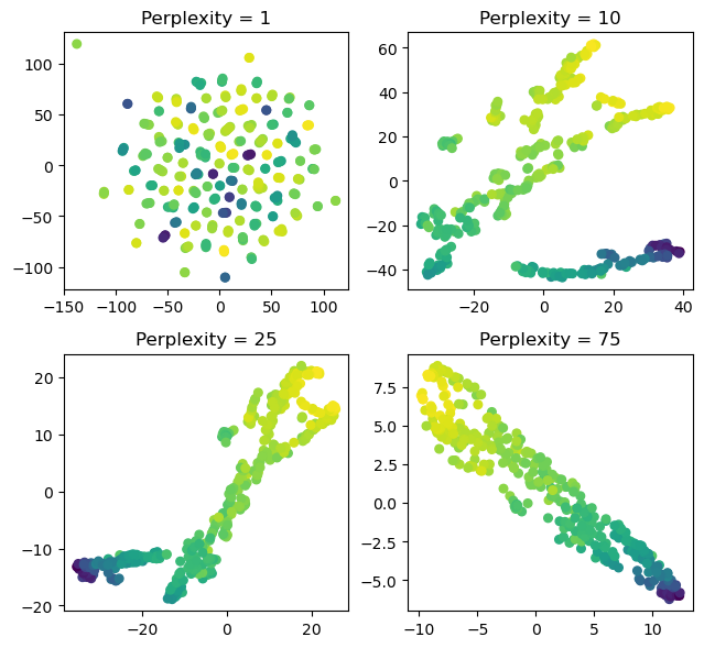
The code below demonstrates how perplexity impacts the differentiation between local and global clustering in t-SNE.

plt.figure(figsize = (6.5,6))
plt.subplots_adjust(top = 1.5)
 
for index, p in enumerate([1, 10, 25, 75]):
 
    tsne = TSNE(n_components = 2, perplexity = p, random_state=42)
    tsne_results = tsne.fit_transform(df)
    tsne1 = pd.DataFrame(tsne_results[:,0])
    tsne2 = pd.DataFrame(tsne_results[:,1])
    
    plt.subplot(2,2,index+1)
    plt.scatter(tsne1, tsne2, c=C, s=30)
    plt.title('Perplexity = '+ str(p))
    
plt.tight_layout()  # Adjust layout to prevent overlap
plt.show()

We observe that the number of clusters is determined by the chosen perplexity. I believe that an appropriate perplexity can be determined through visual inspection.

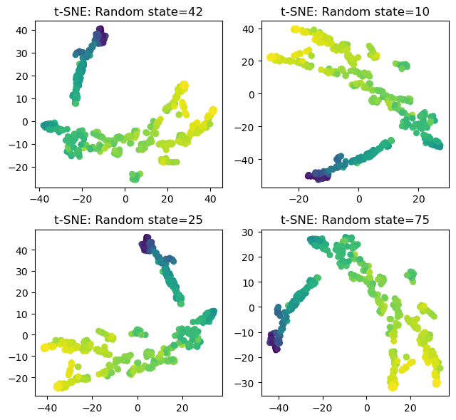
The code below shows the effect of the random states.

plt.figure(figsize = (6.5,6))
plt.subplots_adjust(top = 1.5)
 
for index, r in enumerate([42, 10, 25, 75]):
 
    tsne = TSNE(n_components = 2, perplexity = 15, random_state=r)
    tsne_results = tsne.fit_transform(df)
    tsne1 = pd.DataFrame(tsne_results[:,0])
    tsne2 = pd.DataFrame(tsne_results[:,1])
    
    plt.subplot(2,2,index+1)
    
    plt.scatter(tsne1, tsne2, c=target, s=30)
    plt.title('t-SNE: Random state='+ str(r))
        
plt.tight_layout()  # Adjust layout to prevent overlap
plt.show()

Results of t-SNE can be influenced by different random states, leading to changes resembling rotations, yet it seems that the overall clustering remains relatively unchanged.

From this post, we learn how to use the t-SNE in python. However, I’m not fully knowledgeable about interpreting the results of t-SNE, and I’m currently studying and attempting to apply it to my ongoing research. I believe it would be beneficial if someone well-versed in the t-SNE could offer intuitive explanations in the comments.

Originally posted on SHLee AI Financial Model blog.