Bond Modified Duration in Excel and R

Bond duration is a basic building block for bond portfolio management and asset-liability management (ALM). This post explains the meaning of duration and calculation of this risk measure by using Excel and R.

In this post, a bond price is calculated by discounting future cash flows using YTM which is the abbreviation of Yield To Maturity.

Bond Price

Bond price with unit notional amount, coupon C, YTM y, annual frequency is as follows.

(Modified) Duration

Duration is a measure of price sensitivity to interest rates. At first, we need to calculate an interest rate sensitivity of a bond price.

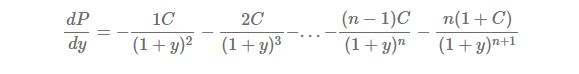
The first derivative of P with respect to y is as follows.

Factoring out in the above equation yields

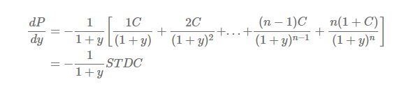
To avoid lengthy expression, we substitute STDC for the bracketed term. STDC is the abbreviation of the sum of multiplications of time and discounted cash flow (only coupon or coupon + principal amount). Of course, this abbreviation is not official

It is noting that the above amount is a kind of a change of bond price. But it is more convenient to use the expression of a percentage change for comparison or analysis. For this reason, let’s modify it by a ratio of its initial bond price.

Through this modification, we can use this measure as a % change of bond price which resulted from a change of interest rate. Dividing by P gives the following expression.

This is the modified duration (D). Modified duration is defined without negative sign since this “minus” sign is popped out of discounting, which indicates that an increase in interest rate lowers a bond price.

Rearranging this equation, we can find that % change of bond price results from the multiplication of modified duration and interest rate change.

For example,

1) If modified duration is 1 (year) and interest rate change is +25bp (= +0.25%), % change of bond price is equal to -0.25% (= -1*0.25%).

2) If modified duration is 10 (year) and interest rate change is +25bp (= +0.25%), % change of bond price is equal to -2.5% (= -10*0.25%).

In other words, the longer the duration or maturity of a bond, the more sensitive is it’s price to a change in interest rates. For this reason, when the central bank increases the target rate, bond portfolio managers have a tendency to make bond portfolio duration shorter to avoid subsequent capital loss due to interest rate hikes. But it is not always.

Macaulay Duration

In fact, Macaulay originally invented the concept of duration. This is called as Macaulay duration which is the average time until receipt of a bond’s cash flows, weighted according to the present values of these cash flows, measured in years.

Interestingly, it is already calculated in the previous equation. Macaulay duration is as follows.

The relationship between modified duration and Macaulay duration is

It is worth while to note that the meaning of “modified” is the modification of Macaulay duration by dividing 1 + y.

As modified duration is widely used than Macaulay duration, when we use the term of duration, it is the modified duration. For this reason, we use D for the modified duration and D_mac for Macaulay duration.

Generalization

When interest conversion period is less than one year such as one quarter, duration is redefined as follows.

Here, k is the number of compounding periods per year.

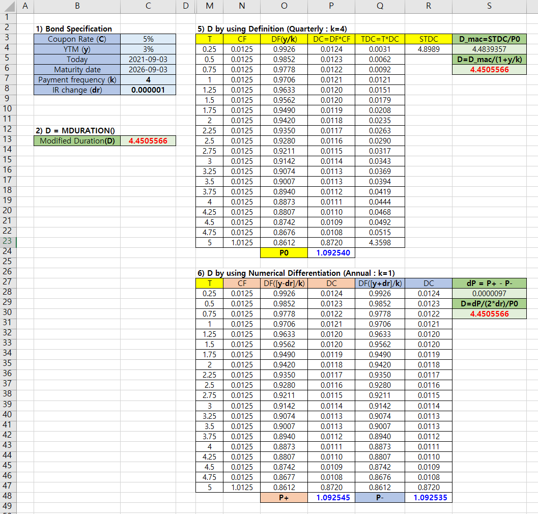
Excel Illustration

Excel provides MDURATION() function for the calculation of modified duration.

    MDURATION (settlement, maturity, coupon, yld, freq)

Arguments of MDURATION() are pricing date, maturity date, coupon rate, YTM, compounding frequency in order.

Besides MDURATION(), we calculate duration by using definition and numerical differentiation for clear understanding.

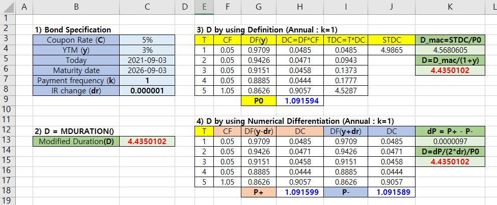
The following Excel spreadsheet shows the case of k=1.

The following Excel spreadsheet shows the case of k=4.

R code

No sooner had we explained the concept of duration than we made the following R code.

#========================================================#
# Quantitative ALM, Financial Econometrics & Derivatives 
# ML/DL using R, Python, Tensorflow by Sang-Heon Lee 
#
# https://shleeai.blogspot.com
#--------------------------------------------------------#
# Bond Modified Duration Calculation
#========================================================#
 
graphics.off()  # clear all graphs
rm(list = ls()) # remove all files from your workspace
 
#-------------------------------------------------------
# Input
#-------------------------------------------------------
    C  <- 0.05       # coupon rate
    y  <- 0.03       # YTM
    m  <- 5          # maturity
    dr <- 0.000001   # interest rate change
 
#-------------------------------------------------------
# Duration by Definition (k=1)
#-------------------------------------------------------
    
    # data.frame for calculation
    df <- data.frame(T = 1:m, 
                     CF = C + c(0,0,0,0,1))
    
    df$DF <- 1/(1+y)^(df$T)
    df$DC <- df$DF*df$CF
    
    P0 <- sum(df$DC) # initial bond price
    
    df$TDC <- df$T*df$DC # time * discounted CF
    
    STDC <- sum(df$TDC)
    
    # duration
    D_mac_dk1 <- STDC/P0         # Macaulay Dur
    D_mod_dk1 <- D_mac_dk1/(1+y) # Modified Dur
    
#-------------------------------------------------------
# Duration by Numerical Differentiation (k=1)
#-------------------------------------------------------
    
    df <- data.frame(T = 1:m, 
                     CF = C + c(rep(0,m-1),1))
    
    df$DFu <- 1/(1+y-dr)^(df$T)
    df$DCu <- df$DFu*df$CF
    
    Pu <- sum(df$DCu) # price up
    
    df$DFd <- 1/(1+y+dr)^(df$T)
    df$DCd <- df$DFd*df$CF
    
    Pd <- sum(df$DCd) # price down
    
    # duration
    D_mod_nk1 <- (Pu-Pd)/(2*dr)/P0 # Modified Dur
    
#-------------------------------------------------------
# Duration by Definition (k=4)
#-------------------------------------------------------
    
    k  <- 4 # Compouding period = Q
    
    df <- data.frame(T = seq(1/k,m,1/k), 
                     CF = C/k + c(rep(0,k*m-1),1))
    
    df$DF <- 1/(1+y/k)^(df$T*k)
    df$DC <- df$DF*df$CF
    
    P0 <- sum(df$DC)
    
    df$TDC <- df$T*df$DC
    STDC <- sum(df$TDC)
    
    D_mac_dk4 <- STDC/P0           # Macaulay Dur
    D_mod_dk4 <- D_mac_dk4/(1+y/k) # Modified Dur
    
#-------------------------------------------------------
# Duration by Numerical Differentiation (k=4)
#-------------------------------------------------------
 
    df <- data.frame(T = seq(1/k,m,1/k),
                     CF = C/k + c(rep(0,k*m-1),1))
 
    df$DFu <- 1/(1+(y-dr)/k)^(df$T*k)
    df$DCu <- df$DFu*df$CF
 
    Pu <- sum(df$DCu)
 
    df$DFd <- 1/(1+(y+dr)/k)^(df$T*k)
    df$DCd <- df$DFd*df$CF
 
    Pd <- sum(df$DCd)
    D_mod_nk4 <- (Pu-Pd)/(2*dr)/P0 # Modified Dur
 
    
    # Print
    cat(paste0("\nDuration Calculation Results \n\n",
        "Macaulay Dur (k=1) def = ", D_mac_dk1, "\n",
        "Modified Dur (k=1) def = ", D_mod_dk1, "\n",
        "Modified Dur (k=1) num = ", D_mod_nk1, "\n",
        "\n",
        "Macaulay Dur (k=4) def = ", D_mac_dk4, "\n",
        "Modified Dur (k=4) def = ", D_mod_dk4, "\n",
        "Modified Dur (k=4) num = ", D_mod_nk4))

The above R code produces the same results as those of Excel exercises.

Duration Calculation Results 
 
Macaulay Dur (k=1) def = 4.56806046946571
Modified Dur (k=1) def = 4.43501016452982
Modified Dur (k=1) num = 4.43501016417148
 
Macaulay Dur (k=4) def = 4.48393573818857
Modified Dur (k=4) def = 4.45055656395888
Modified Dur (k=4) num = 4.45055656459531

Concluding Remarks

From this post, we can understand the meaning of duration, in particular modified duration, by using intuitive derivations and Excel illustrations. Finally we can easily implement R code for the calculation of duration. Upon this work, we can build up the advanced risk management or portfolio optimization model.

But care is taken with some limitation of duration so that duration is the first derivative of highly non-linear bond price function, in other words, or the first order or linearly approximation. To make up for this shortcoming, the second order derivative (convexity) can be considered when the first approximation shows poor result. It depends on the product types and specifications.

Originally posted on SHLee AI Financial Model blog.