Markowitz Model

We present a short article as an insight into the methodology of the Quantpedia Pro report – this time for the Markowitz Portfolio Optimization. As usually, Quantpedia Pro allows the optimization of model portfolios built from the passive market factors (commodities, equities, fixed income, etc.), systematic trading strategies and uploaded user’s equity curves. The current report helps with the calculation of the efficient frontier portfolios based on the various constraints and during various predefined historical periods. The backtests of the periodically rebalanced Minimum-Variance, Maximum Sharpe Ratio and Tangency portfolios will be available at the beginning of July.

Introduction

Markowitz model was introduced in 1952 by Harry Markowitz. It’s also known as the mean-variance model and it is a portfolio optimization model – it aims to create the most return-to-risk efficient portfolio by analyzing various portfolio combinations based on expected returns (mean) and standard deviations (variance) of the assets.

There were several assumptions originally made by Markowitz. The main ones are the following: i) the risk of the portfolio is based on its volatility (and covariance) of returns, ii) analysis is based on a single-period model of investment, and iii) an investor is rational, averse to risk and prefers to increase consumption. Therefore, the utility function is concave and increasing. Additionally, iv) an investor either minimizes their risk for a given return or maximizes their portfolio return for a given level of risk.

When an investor searches for the best portfolio in terms of return-to-risk among the variety of possible portfolios, two steps have to be conducted. The first one is to determine the set of efficient portfolios. The second one is to select the specific, final portfolio from the efficient set, given investor’s target return, target risk or preference toward optimal return-to-risk ratio.

One might ask how to select an optimal portfolio. Basically, from portfolios with the same return, we pick the one with the lowest risk. On the other hand, from portfolios with the same risk level, we choose the one with the highest rate of return.

The efficient portfolios

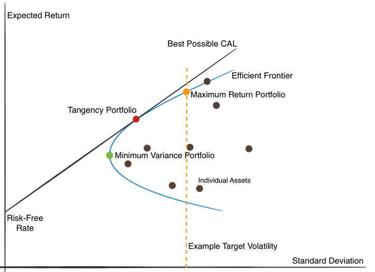
The Efficient Frontier is a hyperbola representing portfolios with all the different combinations of assets that result into efficient portfolios (i.e. with the lowest risk, given the same return and portfolios with the highest return, given the same risk). Risk is depicted on the X-axis and return is depicted on the Y-axis. The area inside the efficient frontier (but not directly on the frontier) represents either individual assets or all of their non-optimal combinations.

Tangency portfolio, the red point in the picture above, is the so-called optimal portfolio that realizes the highest possible Sharpe ratio. As we move from this point either to the right or to the left on the frontier, the Sharpe ratio, or in other words, the excess return-to-risk, will be lower.

The point where the hyperbola changes from convex to concave is where the minimum variance portfolio (green point in the picture) lies.

For a given level of volatility, there also exists a so-called maximum return portfolio (orange point in the picture), which, as the name suggests, maximizes the return given the level of volatility.

Let us now introduce the linear Capital Market Line (CML). The point where the CML meets the Y-axis is where an investor’s risk-free asset, like government securities, lies in terms of the return. This line is tangent to the efficient frontier exactly at the Maximum Sharpe portfolio point. The CML (tangency) line then represents a portfolio of different combinations of a risk-free asset and a tangency portfolio (also called a maximum Sharpe portfolio or sometimes an “optimal portfolio”).

Calculation

When it comes to the math, an efficient frontier can be calculated explicitly, i.e. analytically, only in the simplest case of only one constraint being the sum of asset weights equal to one. Once you start imposing more constraints on asset weights, an optimization procedure needs to be used for calculation of the frontier and the frontier may deviate from the original hyperbola to different curves, given the new constraints. There may be special cases when the solution is explicit, but generally it isn’t.

One of the simplest ways to calculate the efficient frontier under constraints is by using Markowitz’s Critical Line Algorithm (CLA). Unlike some quadratic optimizers, this method works well even if the number of assets N is much greater than the number of observations T. The main idea of CLA is based on a few simple steps. Firstly, you start with the asset with the greatest return, at the upper right side of the Efficient Frontier. Then you follow the Efficient Frontier to the left by looking for the next best asset to be added in or removed one by one.

Numerous curved lines (critical lines), formed by connecting the “corner points”, now form the Efficient Frontier. The portfolios on one critical line, including the corner points, contain same pairs of assets. The only thing that changes are the weights. The set of all critical lines and corner points build up the Efficient Frontier, beginning at the upper right point to the Minimum Variance solution at the far left. Assuming the number of assets, n (n <= N), in the optimal portfolio at a critical line segment is less than the number of observations T (thus n<T), there is a unique solution for CLA.

Visit Quantpedia to read the full article: https://quantpedia.com/markowitz-model.

Past performance is not necessarily indicative of future results.