


In this post I will show how easy it is to price a portfolio of swaps leveraging the purrr package and given the swap pricing functions that we introduced in a previous post. I will do this in a “real world” environment using real market data from April 14.
Import the discount factors from Bloomberg
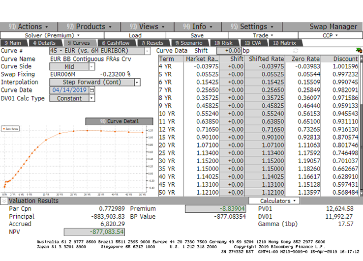
Let’s start the pricing of the swap portfolio with purrr by loading from an external source the EUR discount factor curve. My source is Bloomberg, and in particular the SWPM page, which allows all Bloomberg users to price interest rate sensitive instruments. It also contains a tab with the curve information, which is the source of my curve. It is partly represented in the screenshot below, as well as in the following table:
today <- lubridate::ymd(20190414)
 ir_curve <- readr::read_csv(here::here("data/Basket of IRS/Curve at 140419.csv"))
 ir_curve %>%
 knitr::kable(caption = "Input from Bloomberg", "html") %>%
 kableExtra::kable_styling(bootstrap_options = c("striped", "hover", "condensed", "responsive")) %>%
kableExtra::scroll_box(width = "750px", height = "200px") 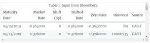
Note: R code and table can be downloaded from Davide’s website:
https://www.curiousfrm.com/2019/04/real-world-tidy-interest-rate-swap-pricing/
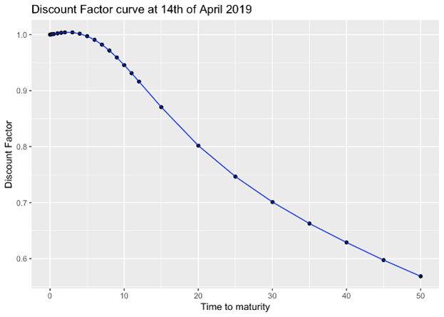
We now wrangle this data in order to get a two-column tibble containing the time to maturity and the discount factors for each pillar points on the curve. We us a 30/360-day count convention because it is the standard for the EUR
df.table <- ir_curve %>%

	dplyr::mutate(`Maturity Date` = lubridate::mdy(`Maturity Date`)) %>%

	dplyr::rowwise(.) %>%

	dplyr::mutate(t2m = RQuantLib::yearFraction(today, `Maturity Date`, 6)) %>%

	na.omit %>%

	dplyr::select(t2m, Discount) %>%

	dplyr::rename(df = Discount) %>%

	dplyr::ungroup(.) %>%

	dplyr::bind_rows(c(t2m = 0,df = 1)) %>%

	dplyr::arrange(t2m)


	ggplot2::ggplot(df.table, ggplot2::aes(x = t2m, y = df)) +

	ggplot2::geom_point() + ggplot2::geom_line(colour = "blue") +

	ggplot2::ggtitle("Discount Factor curve at 14th of April 2019") +

	ggplot2::xlab("Time to maturity") +

	ggplot2::ylab("Discount Factor")
Interest Rate Swap pricing functions
I am now going to re-use the pricing functions that have been already described in a previous post. I have tidied them up a bit and given proper names, but the description still fully holds.
Let’s start from the one that calculates the swap cashflows.
SwapCashflowYFCalculation <- function(today, start.date, maturity.date,

	time.unit, dcc, calendar) {
0:((lubridate::year(maturity.date) - lubridate::year(start.date)) *

	(4 - time.unit)) %>%

	purrr::map_dbl(~RQuantLib::advance(calendar = calendar,

	dates = start.date,

	n = .x, timeUnit = time.unit,

	bdc = 1,

	emr = TRUE)) %>%

	lubridate::as_date() %>% {

if (start.date < today) append(today, .) else .} %>%

	purrr::map_dbl(~RQuantLib::yearFraction(today, .x, dcc)) %>%

	tibble::tibble(yf = .) }
You may have noticed that I added one row {if (start.date < today) append(today, .) else .}. This allows proper management of the pricing of swaps with a starting date before today.
I now proceed with calculating the actual par swap rate, which is a key input to the pricing formula. Notice in the function below that I use a linear interpolation on the log of the discount factors. This is in line with one of the Bloomberg options. It is proven that it:
- provides step constant forward rates
- locally stabilizes the bucketed sensitivities
Also, the (old) swap rate pricing function is the same. We only filter for future cashflows, as we want to be able to price swaps with a starting date before today.
OLDParSwapRate <- function(swap.cf){
 swap.cf %<>%
 dplyr::filter(yf >= 0)

 num <- (swap.cf$df[1] - swap.cf$df[dim(swap.cf)[1]])

 annuity <- (sum(diff(swap.cf$yf)*swap.cf$df[2:dim(swap.cf)[1]]))
return(list(swap.rate = num/annuity,
 annuity = annuity))

 }

 ParSwapRateCalculation <- function(
 swap.cf.yf, df.table) { swap.cf.yf %>%
 dplyr::mutate(df = approx(df.table$t2m, log(df.table$df), .$yf) %>%
 purrr::pluck("y") %>%
 exp) %>%
 OLDParSwapRate
 }
I now want to introduce two new functions which are needed for calculating the actual market values:
- the first one extracts the year fraction for the accrual calculation
- the second one calculates the main characteristics of a swap:
- the par swap rate
- the pv01 (or analytic delta)
- the clean market value
- the accrual for the fixed rate leg
I have defined a variable direction which represents the type of swap:
- if it is equal to
1then it is a receiver swap - if it is equal to
-1then it is a payer swap
CalculateAccrual <- function(swap.cf){

	swap.cf %>% dplyr::filter(yf < 0) %>%

	dplyr::select(yf) %>%

	dplyr::arrange(dplyr::desc(yf)) %>%

	dplyr::top_n(1) %>%
as.double %>%

	{if (is.na(.)) 0 else .}

	}


	SwapCalculations <- function(swap.cf.yf, notional, strike, direction, df.table) {

	swap.par.pricing <- ParSwapRateCalculation(swap.cf.yf, df.table)


	mv <- notional * swap.par.pricing$annuity * (strike - swap.par.pricing$swap.rate) * direction


	accrual.fixed <- swap.cf.yf %>%

	CalculateAccrual %>%

	`*`(notional * strike * direction * -1)


	pv01 <- notional/10000 * swap.par.pricing$annuity * direction

list(clean.mv = mv, accrual.fixed = accrual.fixed, par = swap.par.pricing$swap.rate,

	pv01 = pv01)

	}
We then put everything together with the following pricing pipe:
SwapPricing <- function(today, swap, df.table) {
 SwapCashflowYFCalculation(today, swap$start.date,
 swap$maturity.date, swap$time.unit,
 swap$dcc, swap$calendar) %>%
 SwapCalculations(swap$notional, swap$strike, swap$direction, df.table)
 }
Note: R code can be downloaded from Davide’s website:
https://www.curiousfrm.com/2019/04/real-world-tidy-interest-rate-swap-pricing/
Davide Magno is a professional financial engineer with more than 10 years of experience of managing complex financial quantitative tasks for banks, insurances and funds. He is passionate about both quantitative finance and data science: he is the author of the blog curiousfrm.com that aims at solving financial problems using modern data science coding languages and techniques. He is currently Head of Financial Risk Management in Axa Life Europe dac. Opinions expressed are solely his and do not express the views or opinions of his current employer.
Disclosure: Interactive Brokers
Information posted on IBKR Campus that is provided by third-parties does NOT constitute a recommendation that you should contract for the services of that third party. Third-party participants who contribute to IBKR Campus are independent of Interactive Brokers and Interactive Brokers does not make any representations or warranties concerning the services offered, their past or future performance, or the accuracy of the information provided by the third party. Past performance is no guarantee of future results.
This material is from curiousfrm.com and is being posted with its permission. The views expressed in this material are solely those of the author and/or curiousfrm.com and Interactive Brokers is not endorsing or recommending any investment or trading discussed in the material. This material is not and should not be construed as an offer to buy or sell any security. It should not be construed as research or investment advice or a recommendation to buy, sell or hold any security or commodity. This material does not and is not intended to take into account the particular financial conditions, investment objectives or requirements of individual customers. Before acting on this material, you should consider whether it is suitable for your particular circumstances and, as necessary, seek professional advice.