Risk Parity Asset Allocation

Excerpt

This article is a primer into the methodology we use for the Portfolio Risk Parity report, which is a part of our Quantpedia Pro offering. We explain three risk parity methodologies – Naive Risk Parity (inverse volatility weighted), Equal Risk Contribution and Maximum Diversification. Quantpedia Pro allows the design of model risk parity portfolios built not just from the passive market factors (commodities, equities, fixed income, etc.) but also from systematic trading strategies and uploaded user’s equity curves.

Introduction

Risk parity is an investment management strategy that focuses on risk allocation. The main aim is to find weights of assets that ensure an equal level of risk, most frequently measured by volatility of the portfolio. To allocate the correct “risk parity” weight to an asset, we must understand its risk (and in some variations also return) characteristics. As the simplest benchmark, we use an equally weighted portfolio.

An equally weighted portfolio can be a great choice in many cases; however, when it comes to risk, it has one significant disadvantage. Imagine, we have an equally weighted portfolio consisting of ten assets, of which all but one are highly volatile. In this case, the one low volatile asset brings no diversification benefit. Additionally, the risk contribution of each of the nine highly volatile assets (such as stocks or commodities) is much larger than the risk contribution of the one low volatile asset (such as bonds).

We use simple historical 126-day volatility as a measure of risk. Marginal risk contribution of an asset is calculated as a product of marginal contribution and the weight of the asset divided by 126-day volatility of the portfolio. To find each asset’s marginal contribution, take the cross-product of the weights vector and the covariance matrix divided by 126-day volatility of the portfolio. Portfolio’s diversification ratio is calculated as the ratio between weighted volatility of the assets and volatility of the whole portfolio. The higher the ratio, the more diversified the portfolio.

The following figures show an equally weighted portfolio consisting of SPY (US equities), EFA (EAFE equities), GLD (Gold) and IEF (US 7-10y bonds) ETFs. The figure in the top left shows the weights of the ETFs. As the name suggests, each of the four ETFs has a quarter of the weight in the equally weighted portfolio. The top right figure shows the volatility contribution of each ETF in case of our benchmark equal weight allocation. The bottom left figure shows marginal risk contribution, and the figure in the bottom right shows the diversification ratio.

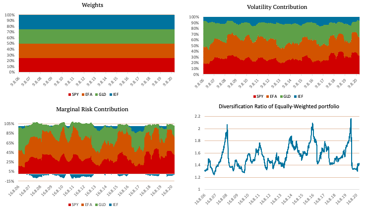
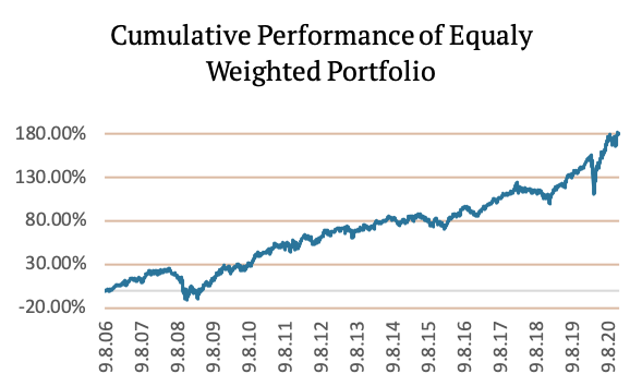
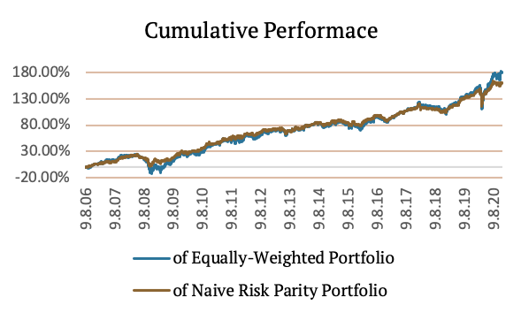
As you can see in the Volatility Contribution graph and the Marginal Risk Contribution graph, the diversification benefit of IEF (US 7-10y bonds) is minimal. Most of the portfolio’s risk is in the SPY (US equities) and EFA (EAFE equities) ETFs. The following figure shows the Cumulative Performance of Equally-Weighted Portfolio.

Naïve Risk Parity

In order to give a low volatile asset an equal opportunity to contribute to a portfolio, we can use naïve risk parity. Naïve risk parity or naïve risk weighting does not use equal weights. Instead, it uses the inverse risk approach. This approach gives lower weight to riskier assets and more significant weight to less risky assets. This method ensures that the risk contribution of each asset is the same.

Theoretically, naïve risk parity is based on the assumption that all the assets in the portfolio have a similar excess return per unit of risk; in other words, have similar Sharpe Ratios. However, the assets’ correlation cannot be determined with high confidence, i.e. it is omitted from the calculation.

There are multiple ways to measure the risk, i.e. input for the risk parity allocation. The most commonly used is volatility; however, variance, Value at Risk (VAR), Conditional Value at Risk (CVar), Conditional Drawdown at Risk (CDaR) or Maximum Daily Loss, and many more can also be used. In the case of normally distributed data, all the listed methods should agree on the optimal asset weights.

Calculating volatility is equal to calculating the standard deviation of daily returns. When the volatility is calculated, we assign the weights using the inverse risk approach:

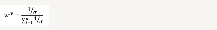
where sigma stands for the vector of asset volatilities.

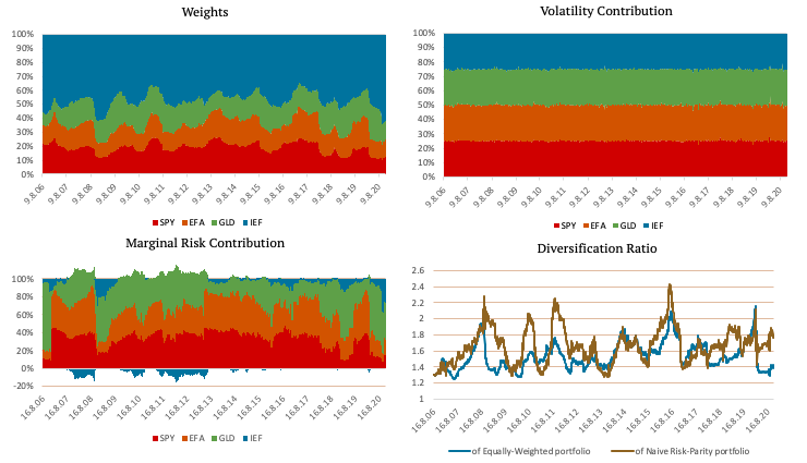
The following figures show a portfolio consisting of SPY, EFA, GLD and IEF ETFs created using Naïve Risk Parity. The top left figure shows the weights of the ETFs. As you can see, the weights are no longer the same. IEF, an ETF consisting of US 7-10y bonds, has the greatest weight, because of its low volatility.

The top right figure shows the volatility contribution of each ETF. The volatility contribution of each ETF is nearly equal when using naïve risk parity. The bottom left figure shows marginal risk contribution, and the figure in the bottom right shows the comparison of diversification ratio of Equally-Weighted portfolio and Naïve Risk-Parity portfolio.

In the following table, we compare the risk metrics of Equally-Weighted portfolio and Naïve Risk-Parity portfolio.

	14Y CAR p.a.	14Y Volatility p.a.	SR	Max DD	95% DD	CAR/ max DD	CAR/ 95% DD
Equally-Weighted Portfolio	7.73%	11.52%	0.67	-29.58%	-14.70%	0.26	0.53
Naive Risk-Parity Portfolio	7.16%	7.33%	0.98	-19.04%	-8.10%	0.38	0.88
Difference	-0.57%	-4.19%	0.31	10.54%	6.60%	0.11	0.36

The following figure shows the Cumulative Performance of Naïve Risk-Parity Portfolio.

Stay tuned for the next installment to learn about Equal Risk Contribution.

Visit Quantpedia for additional insight on this topic: https://quantpedia.com/risk-parity-asset-allocation/.

Past performance is not necessarily indicative of future results.