The Exotic Flavours of Regression in Finance – A First Glance – Part I

Regression is a technique to unearth the relationship between dependent and independent variables. It is routinely seen in machine learning and used mainly for predictive modelling. In the final installment of this series, we expand our scope to cover other types of regression analysis and their uses in finance.

We explore:

• Linear regression
• Simple linear regression
• Multiple linear regression
• Polynomial regression
• Logistic regression
• Quantile regression
• Ridge regression
• Lasso regression
• Comparison between Ridge regression and Lasso regression
• Elastic net regression
• Least angle regression
• Comparison between Multiple Linear regression and PCA
• Comparison between Ridge regression and PCA
• Principal components regression
• Decision trees regression
• Random forest regression
• Support vector regression

---

Previously we have covered the linear regression in great detail. We explored how linear regression analysis can be used in finance,  applied it to financial data, and looked at its assumptions and limitations. Be sure to give them a read.

---

Linear regression

We have covered linear regression in detail in the preceding blogs in this series. We present a capsule version of it here before moving on to the newer stuff. You can skip this section if you’ve spent sufficient time with it earlier.

Simple linear regression

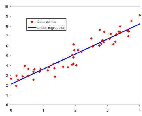
Simple linear regression allows us to study the relationships between two continuous variables- an independent variable and a dependent variable.

Linear regression: Source: https://upload.wikimedia.org/wikipedia/commons/b/be/Normdist_regression.png

The generic form of the simple linear regression equation is as follows:

y_i = β₀ + β₁X_i + ϵ_i                           – (1)

where β₀ is the intercept, β₁ is the slope, and ϵ_i is the error term. In this equation, ‘y’ is the dependent variable, and ‘X’ is the independent variable. The error term captures all the other factors that influence the dependent variable other than the regressors.

Multiple linear regression

We study the linear relationships between more than two variables in multiple linear regression. Here more than one independent variable is used to predict the dependent variable.

The equation for multiple linear regression can be written as:

y_i = β₀ + β₁X_i1 + β₂X_i2 + β₃X_i3 + ϵ_i                                   -(2)

where, β₀, β₁, β₂ and β₃ are the model parameters, and ϵ_i is the error term.

---

Polynomial regression

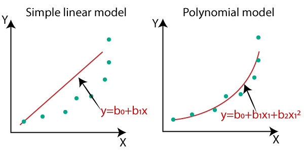
Linear regression works well for modelling linear relationships between the dependent and independent variables. But what if the relationship is non-linear?

In such cases, we can add polynomial terms to the linear regression equation to make it model the data better. This is called polynomial regression. Since the model is linear in parameters, it’s still, strictly speaking, linear regression.

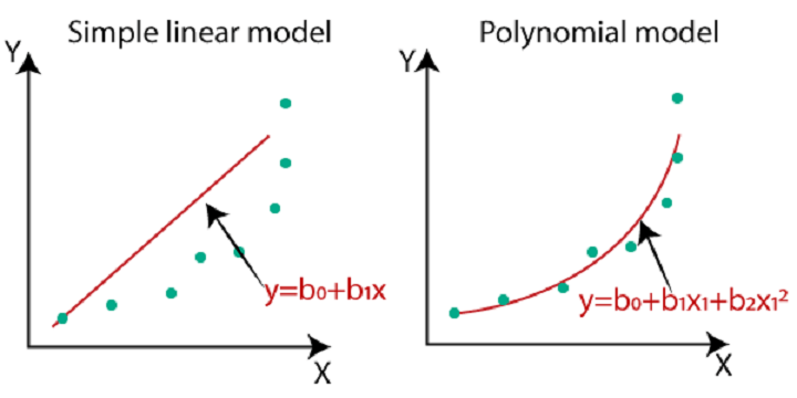
Linear vs Polynomial regression: Source:
https://static.javatpoint.com/tutorial/machine-learning/images/machine-learning-polynomial-regression.png.

Using polynomial regression, we can model the relationship between the independent and dependent variables in the form of a polynomial equation.

The equation for a kth order polynomial can be written as:

y_i = β₀ + β₁X_i + β₂X_i2 + β₃X_i3 + β₄X_i4 + ….. + β_kX_ik + ϵ_i                 -(3)

Choosing the polynomial order is crucial, as a higher degree polynomial could overfit the data. So we try to keep the order of the polynomial model as low as possible.

There are two approaches to choosing the order of the model:

• Forward selection procedure, where we successively fit models in increasing order and test the significance of the coefficients at each iteration till the t-test for the highest order term is not significant.
• Backward elimination procedure, where we start with the highest order polynomial and successively decrease the order in each iteration till the highest order term has a  significant t-statistic.

The most commonly used polynomial regression models are the first- and second-order polynomials.

Polynomial regression is more suited when we have a large number of observations. However, it is sensitive to the presence of outliers.

The polynomial regression model can be used for the prediction of non-linear data like the stock prices. You can read more about polynomial regression and its use in predicting stock prices here.

---

Logistic regression

This is also known as the logit regression. Logistic regression is an analytical method to predict the binary outcome of an occurrence based on past data.

When the dependent variable is qualitative and takes binary values, it is called a dichotomous variable.

If we use linear regression for predicting such a variable, it will produce values outside the range of 0 to 1. Also, since a dichotomous variable can take on only two values, the residuals will not be normally distributed about the predicted line.

Logistic regression is a non-linear model that produces a logistic curve where the values are limited to 0 and 1.

This probability is compared to a threshold value of 0.5 to decide the final classification of the data into one class. So if the probability for a class is more than 0.5, it is labeled as 1, else 0.

One of the use cases of logistic regression in finance is that it can be used to predict the performance of stocks.

You can read more about logistic regression along with Python code on how to use it to predict stock movement on this blog.

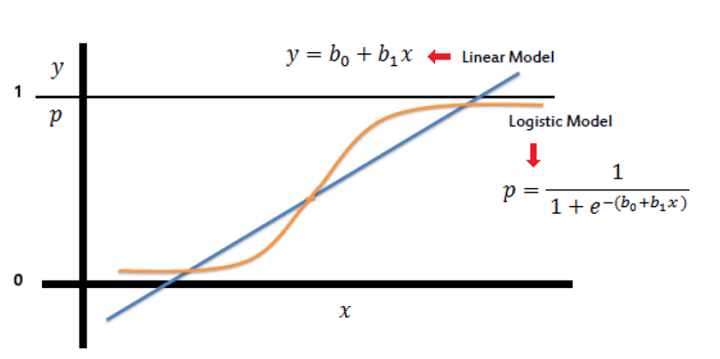
Logistic regression: Source:
https://www.saedsayad.com/logistic_regression.htm.

References

1. Econometrics by example – Damodar Gujarati
2. The basics of financial econometrics – Frank J. Fabozzi, Sergio M. Focardi, Svetlozar T. Rachev, Bala G. Arshanapalli
3. Econometric Data Science – Francis X. Diebold
4. An Introduction to Statistical Learning – Gareth James, Daniela Witten, Trevor Hastie, Robert Tibshirani

Stay tuned for the next installment in which Vivek Krishnamoorthy and Udisha Alok will discuss Quantile regression.

Visit QuantInsti for additional insight on this topic: https://blog.quantinsti.com/types-regression-finance/.