Understanding Logistic Regression

This post explains the logistic regression and implements R code for the estimation of its parameters.

Introduction

Logistic Regression is a benchmark machine learning model. This model have a binary response variable (Y) which takes on 0 or 1. We can find lots of this kind of variables, among them are success/failure, bankruptcy/solvency, exit/stay. To understand logistic regression model, we should know PMF(probability mass function) of the binomial distribution since its log likelihood function is constructed using this PMF. Given this log likelihood function, we can estimate its parameters by maximizing the log likelihood function by MLE (maximum likelihood estimation).

PMF for the binomial distribution

Given success probability p and the number of trials n, binomial distribution produces the probability of occurring x(≤n) success as follows.

From the above equation for P(X=x;n,p),   denotes the case when the number of success is x from n Bernoulli trials. Let’s take an example: suppose n = 3, x = 1.

denotes the probability of . This probability of the above example (n = 3, x = 1) is as follows.

It is worth noticing that since P(X=x;n,p) have one p, the symbol of combination is used. This logic is similar to that of calculating one weighted average.

Standard linear regression is used for the calculation of the conditional mean, which is varying with the realization of covariates (X). This means that in addition to the unconditional mean, additional information from covariates are useful for the improvement of forecast performance. This story is also applied to logistic regression. Assuming p is neither a fixed nor an unconditional probability, we can estimate the conditional probability using explanatory variables (X).

Logit transformation

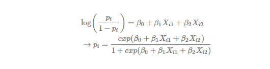
Since explanatory variables X have useful information for explaining variation of a binary variable Y, we can set up a linear regression model for this binary response variable. But output from a standard linear regression can be of less than zero or more than one. This is, therefore, not appropriate because Y is the binary variable which have a range from 0 and 1. From this reason, we need the following logit transformation which converts 0~1 binary variable to −∞~∞ real number.

Using this transformation, we can obtain the logistic regression model in the following way.

Log-likelihood function

Since each 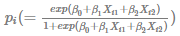 is different with covariates, likelihood function of logistic regression as successive Bernoulli trials, has the following form.

We can find that there is no term like in the likelihood function. The reason is that is different with covariates as mentioned previously. Combination is used only when occurrence probability are fixed and all the same. In particular, to facilitate a numerical optimization, we use the following log likelihood function.

It is typical to estimate parameters using MLE by calling numerical optimization. But for ready-made models like linear regression, logistic regression, etc, it is convenient to use glm() R package which performs optimization automatically.

R code for Logistic Regression

The following R code shows how to implement logistic regression using R. We provide two-method: the one uses glm() conveniently and the other maximize log likelihood function by numerical MLE directly. To check for the accuracy of estimation, we assume population parameters as 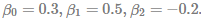. It is, therefore, expected that two methods produce the same results.

#=========================================================================#
# Financial Econometrics & Derivatives, ML/DL using R, Python, Tensorflow  
# by Sang-Heon Lee 
#-------------------------------------------------------------------------#
# Logistic Regression
#=========================================================================#
 
graphics.off()  # clear all graphs
rm(list = ls()) # remove all files from your workspace
 
#-----------------------------------------------------
# Simulated data
#-----------------------------------------------------
 
    # number of observation
    nobs <- 10000
    
    # parameters assumed
    beta <- c(0.3, 0.5, -0.2)
    
    # simulated x
    x1 <- rnorm(n = nobs)
    x2 <- rnorm(n = nobs)
    
    bx = beta[1] + beta[2]*x1 + beta[3]*x2
    p = 1 / (1 + exp(-bx))
    
    # simulated y
    y <- rbinom(n = nobs, size = 1, prob = p)
    
    # simulated y and x
    df.yx <- data.frame(y, x1, x2)      
    
#-----------------------------------------------------
# Estimation by glm
#-----------------------------------------------------
 
    fit_glm = glm(y ~ ., data = df.yx, family = binomial)
    summary(fit_glm)
    
#-----------------------------------------------------
# Estimation by optimization
#-----------------------------------------------------
    
    # objective function = negative log-likelihood
    obj.func <- function(b0, df.yx) {
        
        beta <- b0
        y <- df.yx[,1]
        x <- as.matrix(cbind(1,df.yx[,-1]))
        
        bx = x%*%beta
        p = 1 / (1 + exp(-bx)) 
        
        # we can calculate log-likelihood
        # using one of the two below
        
        # 1. vector operation
        #
        loglike <- sum(y*log(p) + (1-y)*log(1-p))
 
        # 2. loop operation
        #
        # loglike <- 0
        # for(i in 1:nrow(df.yx)) {
        #    loglike <- loglike + y[i]*log(p[i]) + 
        #               (1-y[i])*log(1-p[i])
        # }
 
        return(-1*loglike)
    }
    
    # run optimization
    m<-optim(c(0.1,0.1,0.1), obj.func,
             control = list(maxit=5000, trace=2),
             method=c("Nelder-Mead"),df.yx=df.yx)
    
#-----------------------------------------------------
# Comparison of results
#-----------------------------------------------------
    beta
    m$par
    coef(fit_glm)

The above R program delivers the parameter estimates from two approaches.

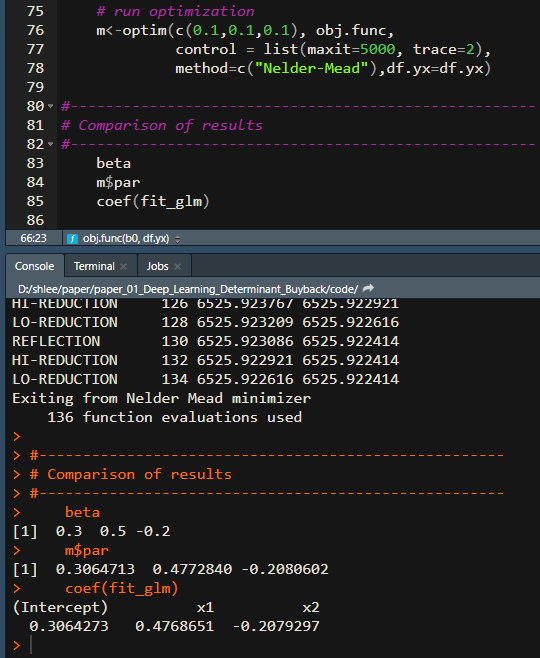
From the estimation output, we can find that two approaches show the same results. Numerical optimziation for MLE is used only for educational purpose. It is, therefore, recommended to use glm() function.

For additional insight on this topic and to download the R script, visit https://kiandlee.blogspot.com/2021/05/understanding-logistic-regression.html.