Value at Risk (VaR) Calculation in Excel and Python

What is the most I can lose on an investment? This is the question every investor who has invested asks at some point in time. Value at Risk (VaR) tries to provide an answer since it is the measurement of the maximum expected loss a portfolio bears.

We will understand and perform VaR calculation in Excel and Python using the Historical Method and Variance-Covariance approach, along with examples with this blog that covers:

• What is VaR?
• Why use VaR?
• Essential points to know while using VaR
• How is VaR calculated in Excel?
• VaR calculation using Variance-Covariance approach
• VaR calculation using the Historical Simulation approach

What is VaR?

Value at Risk or VaR is the measurement of the worst expected loss over a specified period under the usual market conditions. The VaR is measured using ‘confidence levels’ which lie in the range of 90% to 99% such as 90%, 95%, or 99%. The holding period of the financial instrument may vary from a day to a year.

In other words, VaR is a measure of market risk. It is the measure of maximum loss that can occur with a certain confidence interval over a given period of time. Using VaR, financial institutions can determine the sufficient capital reserves they need to cover losses. Also, VaR helps determine whether higher than acceptable risk holdings need to be reduced.

According to Philippe Jorion,
“VaR measures the worst expected loss over a given horizon under normal market conditions at a given confidence level”.

Also, according to one of the studies ⁽¹⁾, it was concluded that ​​VaR does not provide any certainty but rather expectation of outcomes based on certain assumptions.

---

Example

Lets us understand VaR with an example.

Suppose, an analyst says that the 1-day VaR of a portfolio is 1 million dollars, with a 95% confidence level.

• It implies there is a 95% chance that the maximum losses will not exceed 1 million dollars in a single day.
• In other words, there is only a 5% chance that the portfolio losses on a particular day will be greater than 1 million dollars. Learn quantitative portfolio management in detail in the Quantra course.

---

Why use VaR?

Now, let us find out why one uses VaR or Value at Risk for measuring the expected loss. A trader utilises VaR for the following reasons:

• Understanding the Value at Risk result is easy
• Applicable to all asset types
• Universally utilised

Understanding the result of Value at Risk is easy

Value at Risk represents the extent of risk a trader bears for investing in a portfolio in a single figure. For instance, the Value at Risk is between 90% and 99% which makes it easy to interpret the level of risk.

Applicable to all asset types

Vale at Risk can be easily applied to all asset types, namely, bonds, shares, currencies, derivatives, etc. Also, Value at Risk is utilised by all kinds of financial institutions and banks in order to assess the profitability over risk borne for trading a portfolio or asset. Learn Financial Time Series Analysis for Trading in detail in the Quantra course.

Universally utilised

Value at Risk is an accepted standard for basing buying, selling and all trade-related activities. Hence, you can use it anywhere across the globe.

---

Essential points to know while using VaR

There are a couple of essential points that a trader must know while using VaR as the measurement of risk against investment in a portfolio or financial instrument. These points are:

1. VaR is difficult to calculate for portfolios with a diversity of assets (such as cash, currency, stocks etc.) or a greater number of assets

Calculating Value at Risk for a portfolio needs one to calculate the risk and return of each asset. But, along with the risk-return calculation, the correlations between the assets are also to be calculated. Hence, the more the number or diversity of assets in a portfolio, the more difficult it is to calculate VaR.

2. Different methods or approaches lead to varying results

When different approaches to calculating VaR lead to different results for the same portfolio or the financial instrument, it implies the return distribution is not normal.

---

How is VaR calculated in Excel?

There are two well-known methods that are used for VaR calculation.

In this blog, we will discuss the following:

• Variance-covariance approach
• Historical simulation approach

Let’s start with the Variance-Covariance approach.

The Variance-covariance is a parametric method which assumes that the returns are normally distributed. In this method,

• We first calculate the mean and standard deviation of the returns
• According to the assumption, for  95% confidence level, VaR is calculated as a mean -1.65 * standard deviation
• Also, as per the assumption, for 99% confidence level, VaR is calculated as mean -2.58 * standard deviation

Please note that the abovementioned figures are on the basis of a subjective assumption ⁽²⁾.

Moving on, the steps for VaR calculation using the Historical simulation approach are as follows:

1. Similar to the variance-covariance approach, first we calculate the returns of the stock Returns = Today’s Price – Yesterday’s Price / Yesterday’s Price
2. Sort the returns from worst to best.
3. Next, we calculate the total count of the returns.
4. The VaR(90) is the sorted return corresponding to 10% of the total count.
5. Similarly, the VaR(95) and VaR(99) is the sorted return corresponding to the 5% and 1% of the total count respectively.

VaR calculation using Variance-Covariance approach

Now, we will find out the calculation if Variance-Covariance approach using Python.

# We will import the necessary libraries

import numpy as np
import pandas as pd
import yfinance as yf
from tabulate import tabulate

# Plotting
import matplotlib.pyplot as plt
import seaborn
import matplotlib.mlab as mlab

#Statistical calculation
from scipy.stats import norm

# We will import the daily data of Amazon from yahoo finance
# Calculate daily returns
df = yf.download("AMZN", "2020-01-01", "2022-01-01")
df = df[['Close']]
df['returns'] = df.Close.pct_change()


# Now we will determine the mean and standard deviation of the daily returns 
# Plot the normal curve against the daily returns

mean = np.mean(df['returns'])
std_dev = np.std(df['returns'])

df['returns'].hist(bins=40, normed=True, histtype='stepfilled', alpha=0.5)

x = np.linspace(mean - 3*std_dev, mean + 3*std_dev, 100)
plt.plot(x,mlab.normpdf(x, mean, std_dev),"r")
plt.show()

VaR_plot.py hosted with ❤ by GitHub

Output:

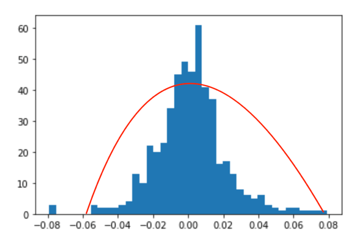
Source: Daily data of Amazon from yahoo finance

# Calculate the VaR using point percentile function
VaR_90 = norm.ppf(1-0.9, mean, std_dev)
VaR_95 = norm.ppf(1-0.95, mean, std_dev)
VaR_99 = norm.ppf(1-0.99, mean, std_dev)
print (tabulate([['90%', VaR_90], ['95%', VaR_95], ['99%', VaR_99]], headers = ['Confidence Level', 'Value at Risk']))

Calculate_VaR.py hosted with ❤ by GitHub

Output:

Confidence Level      Value at Risk (%)
------------------  ---------------
90%                      -0.0245616
95%                      -0.031914
99%                      -0.0457059

The values above imply the confidence level of the particular “value” that is at a risk of being lost. Hence, the confidence rate is 90% that the loss may be -0.0245616 and not more than that.

Similarly, there is a 95% of confidence that the loss of value may be -0.031914 and not more and there is 99% confidence that the loss will go to -0.0457059 and not beyond. Since all the values at risk are in negative, the probability is higher that the portfolio will return more than invested amount.

Visit QuantInsti to read the full article: https://blog.quantinsti.com/calculating-value-at-risk-in-excel-python/