Trend-Following Filters – Part 4

The post “Trend-Following Filters – Part 4” first appeared on Alpha Architect Blog.

Excerpt

1. Introduction

Previous articles in this series examine, from a digital signal processing (DSP) frequency domain perspective, various types of digital filters used by quantitative analysts and market technicians to analyze and transform financial time series for trend-following purposes.

1. An Introduction to Digital Signal Processing for Trend Following
2. Trend-Following Filters – Part 1
3. Trend-Following Filters – Part 2
4. Trend-Following Filters – Part 3

All the filters reviewed in these articles have fixed, time-invariant coefficients and, as a result, are “tuned” to specific frequency responses, precluding them from being able to adjust to the volatility and non-stationarity usually observed in financial time series.

This article and the subsequent Part 5 consider a different type of filter called the Kalman filter. The Kalman filter is a statistics-based algorithm used to perform the estimation of random processes. As an example, a basic random process estimation problem is: Given a discrete-time series of a process:

z(t) = x(t) + ε(t)

where

• x(t) represents the actual underlying value or “state” of the process at each integer time step t which is not directly observable and
• z(t) is the measurement of the process state made at each time step t which is contaminated by additive random normally distributed noise ε(t) where ε(t) ~ N(0, σ_ε²),

then estimate the state values x(t). Estimation of processes in noisy environments is a critical task in many fields, such as communications, process control, track-while-scan radar systems, robotics, and aeronautical, missile, and space vehicle guidance. The Kalman filter is a real-time algorithm used in a variety of complex random process estimation applications.

2. Kalman Filter Overview

This section presents an overview of the Kalman filter. More detailed treatments are available in numerous books, articles, and online resources⁽¹⁾. The algorithm is generally credited to Kalman ⁽²⁾, although Swerling ⁽³⁾ and Stratonovich ⁽⁴⁾ independently developed similar approaches somewhat earlier.

The most commonly-used Kalman filter algorithm, which is described here, operates iteratively in the discrete-time domain (the continuous-time version is called the Kalman-Bucy filter ⁽⁵⁾). The algorithm is based on state-space modeling in which a mathematical model of the process under consideration is represented as a set of input, output, and state variables related by linear difference equations (by linear differential equations in continuous time). The state variables represent the key elements of the process to be estimated. The Kalman filter actually consists of two models:

• a process model of the state variables where the process is contaminated by process noise and
• a measurement model of one or more of the state variables where the measurements (also called “observations”) are contaminated by measurement noise.

Standard Kalman filter process and measurement model equations, variable initialization, and algorithm steps are shown in Appendix 1. Since processes can contain multiple input, output, and state variables, Kalman filter equations are usually stated in matrix form, employing the operations of matrix addition, subtraction, multiplication, transposition (indicated by ^T), and inversion (indicated by ^-1). In the general case, all scalars, vectors, and matrices can potentially be time-varying (indicated by (t)).

The process model consists of:

• a vector X of the state variables,
• an additive process noise vector W ~ N(0, Q) where Q is the covariance of the process noise,
• a process noise input vector G which represents the effects of the process noise vector W at the previous integer time step t-1 on the state vector X at time step t, and
• a state transition matrix F representing a linear model of the process which translates the state vector X at the previous time step t-1 to time step t.

The process model equation shown in Appendix 1 does not include an external process control input term, since it is not relevant in the examples in this article.

The measurement model consists of:

• a measurement input matrix H which maps measurements of the state vector X to the measurement vector Z at time step t and
• an additive measurement noise vector V ~ N(0, R) where R is the covariance of the measurement noise.

A matrix block diagram of the process and measurement models is shown below. The input to the process model is the process noise W(t), and the output is the state vector X(t). The inputs to the measurement model are the state vector X(t) and the measurement noise vector V(t), and the output is the measurement vector Z(t).

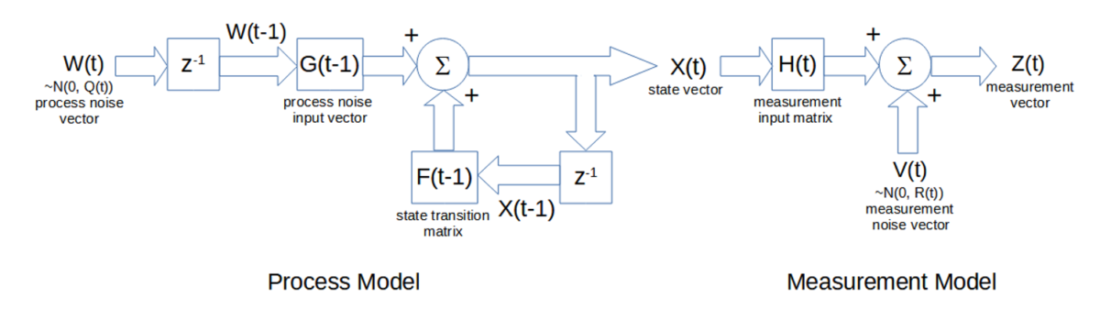
note: the square matrix blocks indicate multiplication of the input by the matrix, the circle Σ blocks indicate matrix addition of the inputs, and the z^-1 blocks represent a unit (i.e., one-time step) delay of the input

Each iteration of the Kalman filter algorithm at each time step t consists of three steps:

1. The time update (also called the “predicted” or “a priori” update) of the state estimate vector, denoted by X^–(t), and of the state estimate covariance matrix, denoted by P^–(t) – The time update X^–(t) projects, from the previous state measurement update X⁺(t-1), the effect of the process between time measurements, as modeled by the state transition matrix F(t-1). Similarly, the covariance time update P^–(t) projects, from the previous covariance measurement update P⁺(t-1), the effect of the process between time measurements, as modeled by the transition matrix F(t-1), in addition to the effect of the previous process noise covariance Q(t-1), based on the process noise input vector G(t-1).
2. The filter gain update of the gain matrix K(t) – The gain matrix K(t) determines the relative weighting used in the subsequent measurement update calculations, based on the relative uncertainties (as indicated by the covariances) of the current state time update P^–(t) versus the current measurement noise R(t). More weight is given to the one with the lower uncertainty (smaller covariance). For example, if P^–(t) is greater than R(t), the gain in the measurement update will give more weight to the latest measurement Z(t) than to the most recent state estimate X^–(t). The filter gains range between 0 and 1.
3. The measurement update (also called the “corrected” or “a posteriori” update) of the state estimate vector, denoted by X⁺(t), and of the state estimate covariance matrix, denoted by P⁺(t) – The measurement update X⁺(t) calculates a weighted sum of the most recent state estimate X^–(t) and the latest measurement Z(t) based on the filter gain K(t). It also updates the covariance P⁺(t) from the time update P^–(t) based on the filter gain. Note that, in addition to the standard form of the covariance measurement update P⁺(t) equation, the Joseph stabilized form, which is less sensitive to computer roundoff errors that can occur and accumulate over multiple iterations of the algorithm, is also shown and is the form used in the examples.

A matrix block diagram of the state estimate time update X^–(t) and measurement update X⁺(t) calculations is shown below. The input is the measurement vector Z(t), and the output is the state estimate measurement update vector X⁺(t).

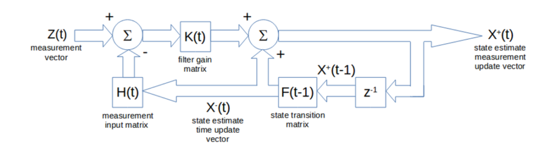
note: the square matrix blocks indicate multiplication of the input by the matrix, the circle Σ blocks indicate matrix addition of the inputs, and the z^-1 block represents a unit (i.e., one-time step) delay of the input

A matrix block diagram of the state estimate covariance time update P^–(t) and standard (non-Joseph stabilized) measurement update P⁺(t) calculations and of the filter gain update K(t) calculations is shown below. The inputs are the process noise covariance Q(t) and the measurement noise covariance R(t). The internal output is the update of the elements of the gain matrix K(t).

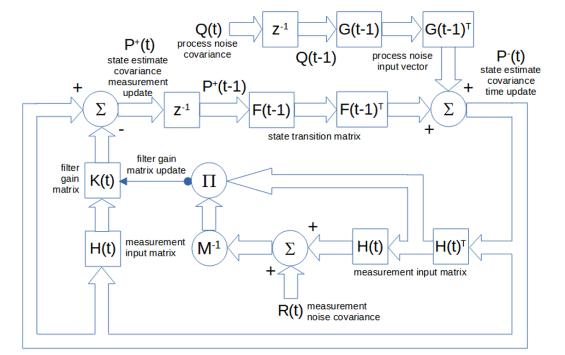
note: the square matrix blocks indicate multiplication of the input by the matrix, including by a transposed matrix denoted by ^T, the circle Σ blocks indicate matrix addition of the inputs, the circle π block indicates matrix multiplication of the inputs, the circle M^-1 block indicates matrix inversion of the input, and the z^-1 blocks represent a unit (i.e., one-time step) delay of the input; the single-line arrow represents an update of the matrix elements

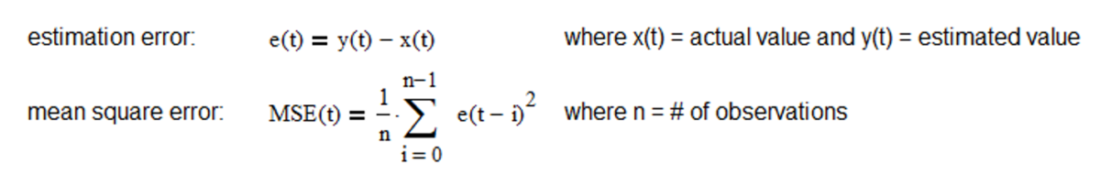
If the process and measurement models are linear and the process and measurement noise covariances are Gaussian, the Kalman filter is the optimal minimum mean square error (MSE) estimator. MSE is the average squared difference between the estimated values and the actual values over a sample of observations and is a statistical measure of the quality of the estimator – the smaller the MSE the better.

If the process and measurement models are linear but the process and measurement noise covariances are not Gaussian, the Kalman filter is the best linear estimator in the MSE sense. Non-linear models can be addressed using the extended Kalman filter or the unscented Kalman filter.

The Kalman filter assumes that the process and measurement noise covariances are known with some accuracy. Inaccurate noise covariance estimates can result in suboptimal state estimates and, in extreme cases, cause filter instability. The Kalman filter algorithm is also sensitive to inaccurate state variable initialization. In practice, the noise covariances, in particular, are often unknown or known only approximately. As a result, the most challenging aspect of Kalman filtering can be estimating the noise covariances.

Visit Alpha Architect Blog to read about Adaptive Kalman Filtering: https://alphaarchitect.com/2022/01/11/trend-following-filters-part-4/