Autocorrelation in Trading: A Practical Python Approach to Analyzing Time Series Data

The article first appeared on on QuantInsti Blog.

Excerpt

Autocorrelation is a statistical concept that measures the correlation between observations of a time series and its lagged values. It is commonly used in various fields, including trading for technical analysis, to identify patterns, trends, and relationships within data.

Autocorrelation helps analyse the dependence between past and present values and provides insights into the persistence or reversibility of data patterns. This helps the trader learn about the trend of stock prices.

All the concepts covered in this blog are taken from this Quantra learning track on Financial time series analysis for trading. You can take a Free Preview of the course by clicking on the green-coloured Free Preview button.

This blog covers:

• What is autocorrelation?
• Example of autocorrelation
• Why is autocorrelation used?
• How does autocorrelation work?
• How to compute autocorrelation?
• How to use autocorrelation with Python in trading?
• Autocorrelation in Technical Analysis
• Autocorrelation vs Partial autocorrelation
• Pros of using autocorrelation
• Cons of using autocorrelation
• FAQs
  • Can machine learning models handle autocorrelation
  • How to detect autocorrelation?
  • What is autocorrelation in econometrics?
  • Is autocorrelation good or bad?
  • Autocorrelation in regression

---

What is autocorrelation?

Autocorrelation refers to the statistical correlation between observations of a time series with their past or future values. In simple terms, It quantifies the similarity or dependence between consecutive data points.

---

Example of autocorrelation

Let us assume a stock price time series where the closing prices for each day are recorded. Autocorrelation in this context would measure the relationship between the closing price on a given day and the closing prices on previous or future days.

Here, you can see the two observations in autocorrelation. It must be noted that autocorrelation can take lags of more days.

The observations are:

• If the closing price today is positively correlated with the closing price of the previous day, it indicates positive autocorrelation and if not it is considered as a negative correlation.
• The positive autocorrelation suggests short-term momentum or trend-following behaviour. Traders can utilise this autocorrelation to identify potential trading opportunities based on the persistence of price movements.

You can see how positive and negative autocorrelation are visualised below.

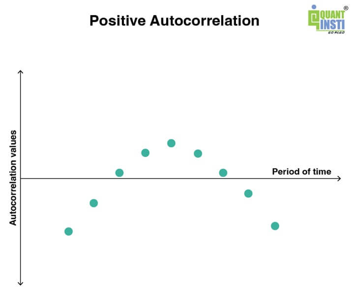
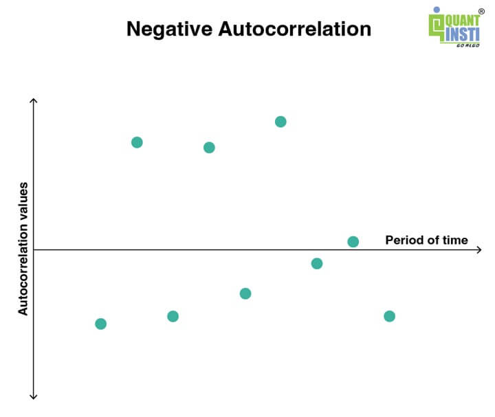
In the image above, the x-axis shows the period of time in years, months etc. Whereas, the y-axis shows the autocorrelation value which we will learn how to compute and utilise ahead in the blog.

---

Why is autocorrelation used?

Autocorrelation is a powerful tool that can enhance your trading skills by enabling you to understand market dynamics, make predictions, manage risk effectively, and develop smarter strategies for more successful trading decisions.

Let us check out some of the uses of autocorrelation in trading below:

• Pattern identification: Autocorrelation enables you to uncover meaningful patterns and relationships in financial data. By comparing past and present market values, you can identify recurring trends and correlations.
• Predicting the future price changes: By studying past autocorrelation patterns, you can gain insights into potential price changes and adjust your trading strategies accordingly.
• Smart strategy development: Leveraging autocorrelation, you can fine-tune your trading strategies by identifying high or low correlation in the mentioned time periods. This knowledge helps you adapt your strategies to capitalise on highly correlated periods for trend-following approaches or low correlation periods for mean-reversion strategies.
• Managing risk: Autocorrelation provides valuable insights into market volatility and stability, allowing you to better manage risk. By assessing the likelihood of price reversals or trend continuations, you can make more informed decisions regarding risk management.

---

Autocorrelation vs Partial autocorrelation

ACF considers both direct and indirect effects, while PACF concentrates exclusively on the direct effect of lagged prices on the current price. PACF helps enhance our understanding of the specific relationships within the time series.

Autocorrelation	Partial autocorrelation
Autocorrelation measures the correlation between a time series observation and its lagged values. It quantifies the linear relationship between an observation and its previous observations at different lags.	Partial autocorrelation measures the direct correlation between an observation and its lagged values, while removing the indirect correlation through intermediate lags.
ACF measures the overall correlation at each lag without considering the influence of intermediate lags. It helps identify the presence of significant patterns and trends in the data.	PACF helps identify the specific lag(s) that directly influence an observation without the influence of other lags. It provides insights into the unique contribution of each lag to the current observation.
ACF is useful for detecting seasonality, identifying the order of an autoregressive (AR) model, and determining the appropriate lag values for forecasting.	PACF is useful for determining the order of a moving average (MA) model, identifying the presence of significant lags, and building autoregressive integrated moving average (ARIMA) models.

---

How does autocorrelation work?

Let us see the working of autocorrelation in a step by step manner. By following the steps below, you can effectively apply autocorrelation analysis to gain insights into the relationship and patterns within your time series data, aiding in decision-making and strategy development.

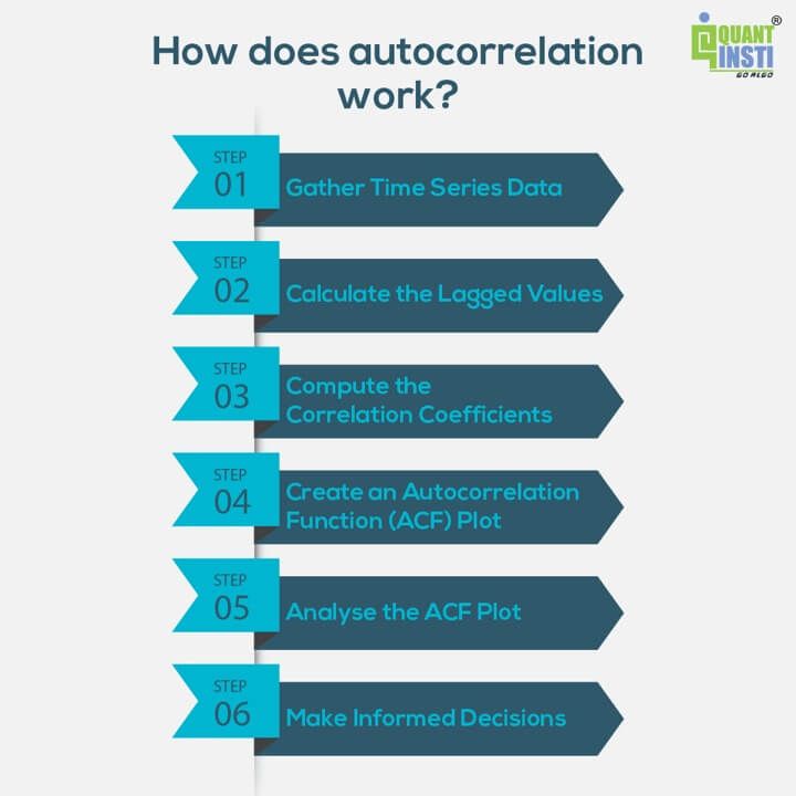
• Gather Time Series Data: Collect the time series data you want to analyse. This could be any sequence of observations recorded at regular intervals, such as stock prices, sales figures, etc.
• Calculate the Lagged Values: For each data point in your time series, determine the lagged values by selecting the previous observations at specific time intervals. Common intervals include one day, one week, one month, or any relevant time frame based on your data.
• Compute the Correlation Coefficients: Calculate the correlation coefficients between the current data point and its corresponding lagged values. The correlation coefficient measures the strength and direction of the relationship.

Common methods for calculating correlation include Pearson correlation or Spearman correlation, depending on the nature of your data.

• Create an Autocorrelation Function (ACF) Plot: Plot the correlation coefficients on the y-axis and the lagged values on the x-axis. This visual representation is known as the Autocorrelation Function (ACF) plot. The ACF plot helps you visualise the correlation patterns and identify significant correlations at different lags.
• Analyse the ACF Plot: Examine the ACF plot to interpret the autocorrelation patterns. Look for significant correlation coefficients at specific lag values. Positive autocorrelation suggests a similar pattern between consecutive data points, while negative autocorrelation indicates an inverse relationship. The magnitude of the correlation coefficient indicates the strength of the relationship.
• Make Informed Decisions: Based on the autocorrelation analysis, make informed decisions regarding your trading or analysis. Positive autocorrelation may indicate a trend-following strategy, while negative autocorrelation may suggest a mean-reversion strategy. Adjust your trading or analytical approach accordingly.

---

How to compute autocorrelation?

To compute autocorrelation, you can follow these steps:

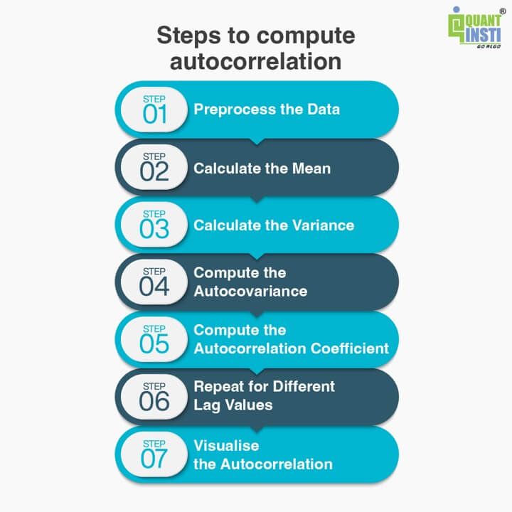
Preprocess the Data

Ensure that your time series data is properly organised and formatted. Remove any missing or irrelevant data points that might interfere with the analysis.

Calculate the Mean

Compute the mean of your time series data. This will be used as a reference point for measuring the correlation between the data points.

Calculate the Variance

Calculate the variance of your time series data. This will help in normalising the autocorrelation values.

Compute the Autocovariance

For each lag value, calculate the autocovariance between the original data points and their corresponding lagged values.

The autocovariance at lag “k” is given by the formula:

Autocovariance(k) = Σ[(X(t) − mean) ∗ (X(t − k) − mean)]/n

Here, X(t) represents the original data point at time “t,” X(t-k) represents the lagged value at time “t-k,” mean is the mean of the data, and “n” is the total number of data points.

Compute the Autocorrelation Coefficient

Normalise the autocovariance values by dividing them by the variance. This yields the autocorrelation coefficient at lag “k.” The autocorrelation coefficient at lag “k” is given by the formula:

Autocorrelation(k) = Autocovariance(k)/Variance

The autocorrelation coefficient ranges from -1 to 1, where -1 represents a perfect negative correlation, 1 represents a perfect positive correlation, and 0 represents no correlation.

Repeat for Different Lag Values

Compute the autocorrelation coefficient for different lag values of interest. This allows you to observe how the correlation changes over time.

Visualise the Autocorrelation

Plot the computed autocorrelation coefficients against the corresponding lag values. This graphical representation is known as the Autocorrelation Function (ACF) plot.

Visit QuantInsti Blog to read about using autocorrelation with Python in trading.