AutoRegressive Moving Average (ARMA) Models: Using R

In the AutoRegressive Moving Average (ARMA) models: A Comprehensive Guide of my ARMA article series, I covered the theoretical aspects of Autoregressive Moving Average models (ARMA). In the AutoRegressive Moving Average (ARMA) models: Using Python, I simulated different ARMA models, their autocorrelations and their partial autocorrelations. We also provided a strategy based on these models. In this article, we’ll do the same as in part 2 but the implementation will be made in R. Let’s enjoy!

We cover:

• Simulation of ARMA models
• Autocovariance and autocorrelation functions in R
• Estimation of the best ARMA model with real-world data in R

---

Simulation of ARMA models

Because there is no second without a third, we have this article to use the ARMA models in R. Let’s code.

Import libraries

First, we install and import the necessary libraries

# Installing the necessary libraries
install.packages('quantmod')
install.packages('TTR')
install.packages('forecast')
install.packages('stats')
# Importing the libraries
library('TTR')
library('quantmod')
library('forecast')
library(stats)

install_and_import_libraries.R hosted with ❤ by GitHub

Create an empty dataframe in R

Then we create an empty dataframe with 1000 rows as previously done in Python.

# Create an empty dataframe
df <- data.frame(matrix(0, ncol = 13, nrow = 1000))

create_empty_dataframe.R hosted with ❤ by GitHub

Simulate ARMA models using R

Next, we simulate the ARMA models as we did before. However, we’re going to make a change. This time we’re going to use the Autoregressive integrated moving average (ARIMA) function provided by the forecast library to create the models.

This is an opportunity to see a different code here in R!

# Set the simulation ARMA parameters
params = c(.1, .25, .5, .75, .9, .99)

# Set the seed
set.seed(2023)

# Use a loop to simulate the ARMA models
for (i in 1:6) {
  # Simulate an AR(p) model based on each parameter
  df[,paste0('X',i)] <-arima.sim(1000, model=list(ar=params[i]))
  # Create the string version of the parameter
  param_string = as.character(params[i])
  # Change the AR(p) model column name
  colnames(df)[i] = paste0("ARMA_1_0_0",substr(param_string,3,nchar(param_string)),"_0")  
  # Simulate an MA(q) model based on each parameter
  df[,paste0('X',(i+6))] <-arima.sim(1000, model=list(ma=-params[i]))
  # Change the MA(q) model column name
  colnames(df)[(i+6)] = paste0("ARMA_0_1_0_0",substr(param_string,3,nchar(param_string)))  }

# Create an ARMA(1,1) model
df[,paste0('X',13)] <-arima.sim(1000, model=list(ar=0.3, ma=-0.3))

# Change the ARMA(1,1) model column name
colnames(df)[13] = paste0("ARMA_1_0_03_03") 

create_simulated_arma_models.R hosted with ❤ by GitHub

Suggested Reads:

• Autocorrelation and Autocovariance: Calculation, Examples, and More
• How to Get Historical Market Data Through Python Stock API

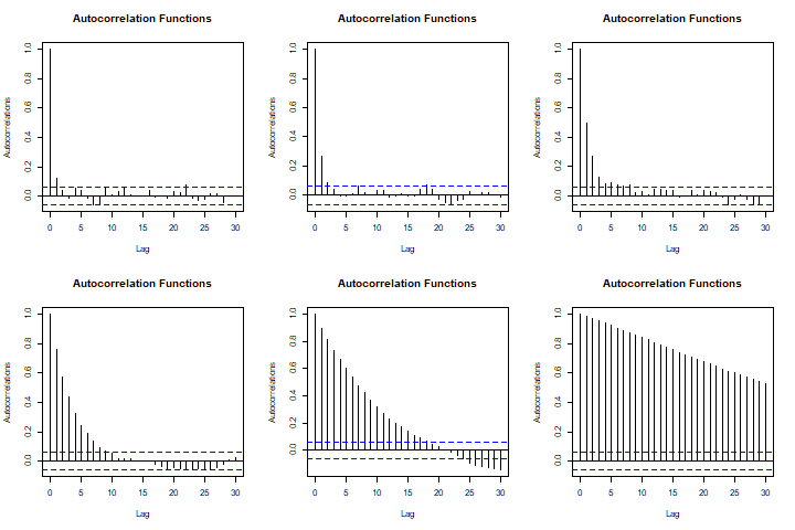
Autocovariance and autocorrelation functions in R

Last but not least, this time we’re going to plot the Autocorrelation function (ACF) and Partial Autocorrelation Function (PACF) of only the Autoregressive (AR) models.

 Create a plot object with 2x3 dimensions
p <- par(mfrow=c(2,3))
# Set the each plot margin sizes
p.par(mar=c(1,1,1,1))
# Create a loop to plot each AR(p) autocorrelation plot
for (i in 1:6) {
  # Create the string version of the parameter value
  param_string <- as.character(params[i])
  # Plot the autocorrelation function
  acf(df[,paste0("ARMA_1_0_0",substr(param_string,3,nchar(param_string)),"_0")],plot= TRUE, xlab = "Lag", ylab = 'Autocorrelations',main = "Autocorrelation Functions", font.main=70) }
par(p)
dev.off()

# Create a plot object with 2x3 dimensions
p <- par(mfrow=c(2,3))
# Set the each plot margin sizes
p.par(mar=c(1,1,1,1))
# Create a loop to plot each ARMA autocorrelation plot
for (i in 1:6) {
  # Create the string version of the parameter value
  param_string <- as.character(params[i])
  # Plot the autocorrelation function
  acf(df[,paste0("ARMA_1_0_0_0",substr(param_string,3,nchar(param_string)))],plot= TRUE, type = 'partial', xlab = "Lag", ylab = 'Autocorrelations',main = "Autocorrelation Functions", font.main=70) }
par(p)
dev.off()

acf_and_pacf_of_ar_models.R hosted with ❤ by GitHub

Check the plots

We leave it as an exercise to plot the same graphs for the MA processes.

Stay tuned for the next installment for estimation of the best ARMA model with real-world data in R.

Originally posted on QuantInsti blog.