How to Build a Logistic Regression Model from Scratch in R

Originally posted on TheAutomatic.net.

Excerpt

Background

In a previous post, we showed how using vectorization in R can vastly speed up fuzzy matching. Here, we will show you how to use vectorization to efficiently build a logistic regression model from scratch in R. Now we could just use the caret or stats packages to create a model, but building algorithms from scratch is a great way to develop a better understanding of how they work under the hood.

Definitions & Assumptions

In developing our code for the logistic regression algorithm, we will consider the following definitions and assumptions:

x = A dxn matrix of d predictor variables, where each column x_i represents the vector of predictors corresponding to one data point (with n such columns i.e. n data points)

d = The number of predictor variables (i.e. the number of dimensions)

n = The number of data points

y = A vector of labels i.e. y_i equals the label associated with x_i; in our case we’ll assume y = 1 or -1

Θ = The vector of coefficients, Θ₁, Θ₂…Θ_d trained via gradient descent. These correspond to x₁, x₂…x_d

α = Step size, controls the rate of gradient descent

Logistic regression, being a binary classification algorithm, outputs a probability between 0 and 1 of a given data point being associated with a positive label. This probability is given by the equation below:

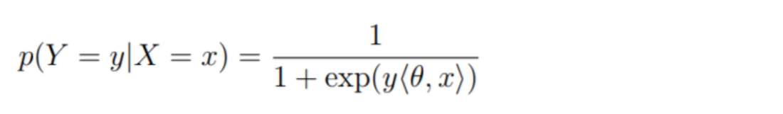
Recall that <Θ, x> refers to the dot product of Θ and x.

In order to calculate the above formula, we need to know the value of Θ. Logistic regression uses a method called gradient descent to learn the value of Θ. There are a few variations of gradient descent, but the variation we will use here is based upon the following update formula for Θ_j:

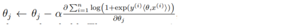
This formula updates the j^th element of the Θ vector. Logistic regression models run this gradient descent update of Θ until either 1) a maximum number of iterations has been reached or 2) the difference between the current update of Θ and the previous value is below a set threshold. To run this update of theta, we’re going to write the following function, which we’ll break down further along in the post. This function will update the entire Θ vector in one function call i.e. all j elements of Θ.

# function to update theta via gradient descent
update_theta <- function(theta_arg,n,x,y,d,alpha)
{
   
  # calculate numerator of the derivative
  numerator <- t(replicate(d , y)) * x
   
  # perform element-wise multiplication between theta and x,
  # prior to getting their dot product
  theta_x_prod <- t(replicate(n,theta_arg)) * t(x)
  dotprod <- rowSums(theta_x_prod)
   
  denominator <- 1 + exp(-y * dotprod)
   
  # cast the denominator as a matrix
  denominator <- t(replicate(d,denominator)) 
   
  # final step, get new theta result based off update formula
  theta_arg <- theta_arg - alpha * rowSums(numerator / denominator) 
   
   
  return(theta_arg)
   
}

Simplifying the update formula

To simplify the update formula for Θ_j, we need to calculate the derivative in the formula above.

Let’s suppose z = (y_i)(<Θ, x_i>). We’ll abbreviate the summation of 1 to n by simply using Σ.

Then, calculating the derivative gives us the following:

Σ (1 / exp(1 + z)) * exp(z) * x_iy_i

= Σ (exp(z) / exp(1 + z)) * x_iy_i

Since exp(z) / (1 + exp(z)) is a known identity for 1 / (1 + exp(-z)), we can substitute above to get:

Σ 1 / (1 + exp(-z)) * x_iy_i

= Σ x_iy_i / (1 + exp(-z))

Now, substituting (y_i)(<Θ, x_i>) back for z:

= Σ x_iy_i / (1 + exp(-(y_i)(<Θ, x_i>)))

Plugging this derivative result into the rest of the update formula, the below expression tells us how to update Θ_j:

Θ_j ← Θ_j – αΣ x_iy_i / (1 + exp(-(y_i)(<Θ, x_i>)))

To convert this math into R code, we’ll split up the formula above into three main steps:

• Calculate the numerator: x_iy_i
• Calculate the denominator: (1 + exp(-(y_i)(<Θ, x_i>)))
• Plug the results from first two steps back into the formula above

The idea to keep in mind throughout this post is that we’re not going to use a for loop to update each j^th element of Θ. Instead, we’re going to use vectorization to update the entire Θ vector at once via element-wise matrix multiplication. This will vastly speed up the gradient descent implementation.

Step 1) Calculating the numerator

In the numerator of the derivative, we have the summation of 1 to n of y_i times x_i. Effectively, this means we have to calculate the following:

y₁x₁ + y₂x₂…+y_nx_n

This calculation needs to be done for all j elements in Θ to fully update the vector. So, we actually need to run the following calculations:

y₁x_1,1 + y₂x_1,2…+y_nx_1,n

y₁x_2,1 + y₂x_2,2…+y_nx_2,n

…

y₁x_d,1 + y₂x_d,2…+y_nx_d,n

Since y is a vector, or put another way, is an nx1 matrix, and x is a dxn matrix, where d is the number of predictor variables i.e. x₁, x₂, x₃…x_d, and n is the number of labels (how many predicted values we have), then we can compute the above calculations by creating a dxn matrix where each row is a duplicate of y. This way we have d duplicates of y. Each ith element of x (i.e. x_i) corresponds to the i^th column of x. So x_j,i refers to the element in the j^th row and i^th column of x.

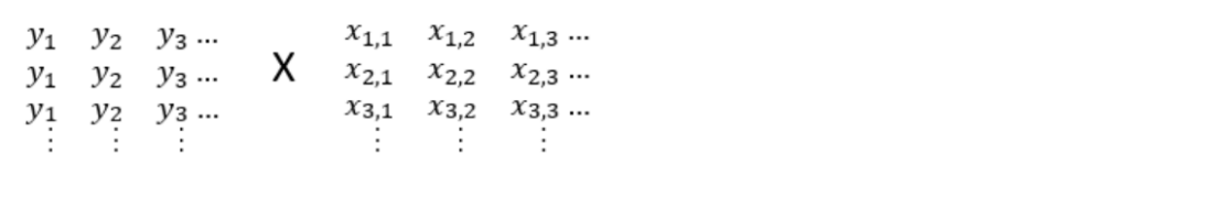
In the above expression, instead of doing traditional matrix multiplication, we are going to do element-wise multiplication i.e. the j^th, i^th element of the resultant matrix will equal the j^th, i^th elements of each matrix multiplied by each other. This can be done in one line of R code, like below:

# calculate numerator of the derivative of the loss function
numerator <- t(replicate(d , y)) * x

Initially we create a matrix where each column is equal to y₁, y₂,…y_n. This is replicate(d, y). We then transpose this so that we can perform the element-wise multiplication described above. This element-wise multiplication gets us the following dxn matrix result:

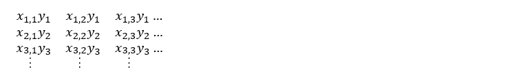
Notice how the sum of each j^th row corresponds to the each calculation above i.e. the sum of row 1 is Σx_iy_i for j = 1, the sum of row 2 is Σx_iy_i for j = 2…the sum of row d is Σx_iy_i for j = d. Rather then using slower for loops, this allows us to calculate the numerator of the derivative given above for each element (Θ_j) in Θ using vectorization. We’ll postpone doing the summation until after we’ve calculated the denominator piece of the derivative.

Visit TheAutomatic.net to read how to calculate the denominator.