How to Create Kalman Filter in Python

If we had to explain Kalman Filter in one line, we would say that it is used to provide an accurate prediction of a variable which cannot be directly measured. In fact, one of the earliest uses of the Kalman filter was to calculate the position of the Apollo space rockets by NASA to make sure it was on the right path.

But how is it applicable in trading? Well, we can use Kalman Filter to implement pairs trading, or even find arbitrage opportunities in the Futures market. But before we start the applications of Kalman filters, let us understand how to use it. Thus, in this blog we will cover the following topics:

• Statistical terms and concepts used in Kalman Filter
• Equations in Kalman Filter
• Pairs trading using Kalman Filter in Python

As such, Kalman filter can be considered a heavy topic when it comes to the use of math and statistics. Thus, we will go through a few terms before we dig into the equations. Feel free to skip this section and head directly to the equations if you wish.

Statistical terms and concepts used in Kalman Filter

Kalman Filter uses the concept of a normal distribution in its equation to give us an idea about the accuracy of the estimate. Let us step back a little and understand how we get a normal distribution of a variable.

Let us suppose we have a football team of ten people who are playing the nationals. As part of a standard health check-up, we measure their weights. The weights of the players are given below.

Player Number	1	2	3	4	5	6	7	8	9	10
Weight	72	75	76	69	65	71	70	74	76	72

Now if we calculate the average weight, ie the mean, we get the value as (Total of all player weights) / (Total no. of players)

= 720/10 = 72

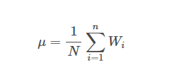
The mean is usually denoted by the Greek alphabet μ. If we consider the weights as w₁, w₂ respectively and the total number of players as N, we can write it as: μ = (w₁ + w₂+ w₃+ w₄+…..+ w_n)/N

Or

Now, on a hunch, we decide on seeing how much each player’s weight varies from the mean. This can be easily calculated by subtracting the individual’s weight from the mean value.

Now, the first team player’s weight varies in the following manner, (Individual player’s weight) – (Mean value) = 72 – 72 = 0.

Similarly, the second player’s weight varies by the following: 75 – 72 = 3. Let’s update the table now.

Player Number	1	2	3	4	5	6	7	8	9	10
Weight	72	75	76	69	65	71	70	74	76	72
Difference from mean	0	3	4	-3	-7	-1	-2	2	4	0

Now, we want to see how much the entire team’s weights’ varies from the mean. A simple addition of the entire team’s weight difference from the mean would be 0 as shown below. Thus we square each individual’s weight difference and find the average. Squaring is done to eliminate the negative sign of a score + penalise greater divergence from mean.

The updated table is as follows:

Player Number	1	2	3	4	5	6	7	8	9	10
Weight	72	75	76	69	65	71	70	74	76	72
Difference from mean	0	3	4	-3	-7	-1	-2	2	4	0
Squared difference from the mean	0	9	16	9	49	1	4	4	16	0

Now if we take the average, we get the equation as,

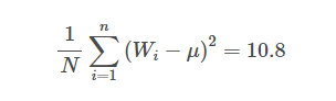
The variance tells us how much the weights have been spread. Since the variance is the average of the squares, we will take the square root of the variance to give us a better idea of the distribution of weights. We call this term the standard deviation and denote it by σ.

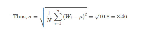
Since standard deviation is denoted by σ, the variance is denoted by σ^2.

But why do we need standard deviation? While we calculated the variance and standard deviation of one football team, maybe we could find for all the football teams in the tournament, or if we are more ambitious, we can do the same for all the football teams in the world. That would be a large dataset.

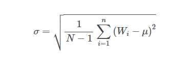
One thing to understand is that for a small dataset w used all the values, ie the entire population to compute the values. However, if it is a large dataset, we usually take a sample at random from the entire population and find the estimated values. In this case, we replace N by (N-1) to get the most accurate answer as per Bessel’s correction. Of course, this introduces some error, but we will ignore it for now.

Thus, the updated equation is,

Now, looking at different researches conducted in the past, it was found that given a large dataset, most of the data was concentrated around the mean, with 68% of the entire data variables coming within one standard deviation from the mean.

This means that if we had data about millions of football players, and we got the same standard deviation and variance which we received now, we would say that the probability that the player’s weight is +-3.46 from 72 kg is 68.26%. This means that 68.26% of the players’ weights would be from 68.53 kg to 75.46.

Of course, for this to be right, the data should be random.

Let’s draw a graph to understand this further. This is just a reference of how the distribution will look if we had the weights of 100 people with mean as 72 and standard deviation as 3.46.

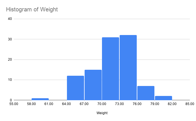
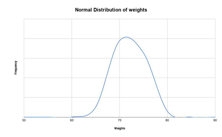
This shows how the weights are concentrated around the mean and tapers off towards the extremes. If we create a curve, you will find that it is shaped like a bell and thus we call it a bell curve. The normal distribution of the weights with mean as 72 and standard deviation as 3.46 will look similar to the following diagram.

Normal distribution is also called a probability density function. While the derivation is quite lengthy, we have certain observations regarding the probability density function.

One standard deviation contains 68.26% of the population.

Two standard deviations contain 95.44% of the population while three contain 99.74%.

The probability density function is given as follows,

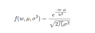
You can find out more about probability density function in this blog. The reason we talked about normal distribution is that it forms an important part in Kalman filters. Let’s now move on to the main topic in the next section of the Kalman filter tutorial.

Stay tuned for the next installment, in which the Rekhit will explain how to create equations in Kalman Filters.

Download the full code: https://blog.quantinsti.com/kalman-filter/.