Johansen Cointegration Test: Learn How to Implement it in Python

Updated by Chainika Thakar (Originally written by Devang Singh)

Time series data is a unique and invaluable form of data that captures information over a continuous period. It’s used in various fields, from finance to economics, to understand and predict trends, patterns, and behaviours.

Among the essential tools for analysing time series data is the Johansen Cointegration Test, which plays a pivotal role in understanding relationships between variables. This blog aims to provide a comprehensive and beginner-friendly guide to mastering the Johansen Cointegration Test using Python.

We’ll embark on this journey by first understanding the core concepts of time series data. What makes it different from other types of data, and how do we extract meaningful insights from it?

In this blog post, you will understand the essence of the Johansen Test for cointegration and learn how to implement it in Python. Another popular test for cointegration is the Augmented Dickey-Fuller (ADF) test. The ADF test has limitations which are overcome by using the Johansen test.

The ADF test enables one to test for cointegration between two-time series. The Johansen Test can be used to check for cointegration between a maximum of 12-time series.

This implies that a stationary linear combination of assets can be created using more than a two-time series, which could then be traded using mean-reverting strategies like Pairs Trading, Triplets Trading, Index Arbitrage and Long-Short Portfolio.

Whether you’re a novice or an aspiring data analyst, this blog will empower you to harness the potential of time series data with the Johansen Cointegration Test.

Some of the concepts covered in this blog are taken from this Quantra course on Mean Reverting Strategies in Python by Dr. E P Chan. You can take a Free Preview of the course.

This blog covers:

• What is the Johansen cointegration test?
• Key properties of Johansen cointegration test
• Importance of Johansen cointegration test
• Applying cointegration in trading or forecasting
• Implementation of Johansen cointegration test with Python
• Tips for successful cointegration analysis

---

What is the Johansen cointegration test?

The Johansen Cointegration Test is a statistical procedure used to analyse the long-term relationships between multiple time series variables. Time Series is a sequence of observations over time, which are usually spaced at regular intervals. For example, daily observed prices of the stocks, bonds etc. over a period of 10 years, 1 minute stock price data for the last 100 days etc.

---

Key properties of Johansen cointegration test

The Johansen Cointegration Test is a valuable tool for economists, financial analysts, and researchers to assess the relationships between multiple time series variables and make informed decisions based on their long-term behaviour.

Key properties of the Johansen Cointegration Test include:

• Multivariate Approach: Unlike some other cointegration tests, the Johansen Test can handle multiple time series variables simultaneously. This makes it especially useful when you want to analyse the relationships between more than two variables.
• Eigenvalues and Eigenvectors: The test relies on the eigenvalues and eigenvectors of a matrix derived from the time series data. These mathematical properties help determine the number of cointegrating relationships between the variables.
• Trace and Maximum Eigenvalue Tests: The Johansen Test consists of two different tests: the Trace test and the Maximum Eigenvalue test. These tests help determine the rank of the cointegration matrix, which, in turn, indicates the number of cointegrating relationships present.
• Order of Integration: The test takes into account the order of integration of the time series variables, allowing it to differentiate between I(0) (stationary) and I(1) (integrated of order 1) series. This is crucial for understanding whether the variables have a common stochastic trend.
• Critical Values: The interpretation of the test results involves comparing test statistics to critical values from statistical tables, which depend on the significance level chosen for the test. These critical values help determine whether cointegration exists.
• Interpretation: The test results can reveal whether there are long-term relationships between the variables. If cointegration is detected, it implies that the variables move together in the long run, and deviations from this equilibrium relationship are mean-reverting.

---

Importance of Johansen Cointegration Test

The Johansen Cointegration Test holds significant importance in the fields of econometrics, finance, and time series analysis for several key reasons:

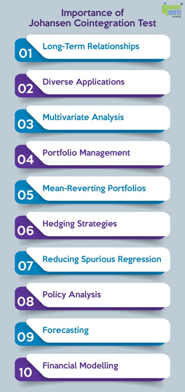
• Long-Term Relationships: It identifies and quantifies the existence of long-term or equilibrium relationships between multiple time series variables. This is crucial for understanding how different economic or financial factors interact over extended periods.
• Diverse Applications: The test can be applied in various contexts, such as finance, economics, and social sciences. It’s used to analyse the relationships between macroeconomic variables, financial instruments, asset pricing models, and more.
• Multivariate Analysis: Unlike some other cointegration tests, the Johansen Test can handle multiple variables simultaneously, making it a versatile tool for analysing complex relationships within a dataset.
• Portfolio Management: In finance, the test is essential for portfolio management. It helps investors and fund managers assess the cointegration of assets in a portfolio, which can inform diversification and risk management strategies.
• Mean-Reverting Portfolios: The test can identify mean-reverting (stationary) portfolios. In such cases, deviations from the long-term equilibrium are expected to return to that equilibrium, making it valuable for traders and investors.
• Hedging Strategies: For hedging purposes, it is important to determine if there are cointegrated relationships between assets or financial instruments. A cointegrated relationship can be exploited for hedging purposes.
• Reducing Spurious Regression: Cointegration analysis helps reduce the risk of spurious regression, a common issue when dealing with non-stationary time series data. By identifying cointegration, researchers avoid drawing erroneous conclusions from non-causal relationships.
• Policy Analysis: In economics, the Johansen Cointegration Test is useful for policy analysis. It can help assess the long-term impact of various economic policies on different variables, providing insights for policymakers.
• Forecasting: Cointegrated variables can be used to improve the accuracy of economic and financial forecasts. By understanding how variables move together in the long term, forecasts can be refined.
• Financial Modelling: The test plays a crucial role in the development of financial models, particularly those involving multiple interacting variables. It enhances the accuracy of models by capturing the underlying cointegrated relationships.

In summary, the Johansen Cointegration Test is a valuable tool for analysing the long-term relationships between time series variables, providing insights into economic and financial dynamics, portfolio management, and policy analysis, among other applications. Its ability to handle multivariate data makes it a versatile and indispensable technique for researchers and practitioners in these fields.

---

Applying cointegration in trading or forecasting

Cointegration, a concept in time series analysis, is especially useful in the world of trading and forecasting. It helps traders and analysts make better predictions and strategic decisions.

Here’s how it works:

• Identifying Trading Pairs: Traders often look for pairs of assets or securities that move together in the long run. Cointegration can help identify these pairs. For instance, if you’re trading stocks, you might notice that the prices of two companies tend to follow a similar pattern over time. These pairs could be useful for a trading strategy.
• Statistical Arbitrage: Cointegration enables traders to engage in statistical arbitrage. This means taking advantage of temporary price divergences within cointegrated pairs. If one stock temporarily deviates from the other in a predictable way, traders can buy or sell to capture the difference when the prices realign.
• Risk Management: Cointegration can be a tool for risk management. By diversifying your investments in cointegrated assets, you can reduce your portfolio’s exposure to risk. When one asset in a pair fluctuates, the other tends to balance it out.
• Forecasts: Cointegration can improve forecasting accuracy. When two or more variables are cointegrated, their long-term relationship can be used to make better predictions. For instance, in economics, cointegrated variables can help in predicting future inflation or interest rates.
• Hedging: Cointegrated assets are often used for hedging purposes. If you have an asset exposed to a certain risk, you can use another cointegrated asset to hedge that risk. This helps protect your investments.

---

Implementation of Johansen cointegration test with Python

This Python code aims to perform the Johansen Cointegration Test for multiple stock pairs, shedding light on their long-term relationships and potential trading strategies.

The pairs of stocks in the code are:

• AAPL (Apple Inc.) and AMZN (Amazon.com, Inc.)
• MSFT (Microsoft Corporation) and AAPL (Apple Inc.)
• AMZN (Amazon.com, Inc.) and MSFT (Microsoft Corporation)

We will find out if each pair is cointegrated or not on the basis of “Testing for Zero Cointegrating Relationships (Null Hypothesis)”. This means that the null hypothesis will be rejected when a pair of stocks is cointegrated.

Let us begin with the code now.

Step 1: Import necessary libraries

# Import libraries
import numpy as np
import pandas as pd
from pandas_datareader import data as pdr
import yfinance as yf
from statsmodels.tsa.vector_ar.vecm import coint_johansen

Libraries.py hosted with ❤ by GitHub

Step 2: Fetch data

Now, we will fetch data for three stocks.

# Set the stock list
stock_list = ['AAPL', 'AMZN', 'NFLX']

# Set the start date and the end date
start_date = '2010-01-01'
end_date = '2022-10-16'

Stock_list.py hosted with ❤ by GitHub

Step 3: Conduct Johansen cointegration test

Now, we will extract the trace statistics and eigen statistics. These statistics are the key components of the Johansen Cointegration Test. We will discuss them later after the output is generated.

# Create a data frame df to store the two-time series
data = yf.download(stock_list, start=start_date, end=end_date)['Adj Close']

# Perform the Johansen Cointegration Test with a specified number of zero
specified_number = 0  # Testing for zero cointegrating relationships
coint_test_result = coint_johansen(data, specified_number, 1)

# Extract the trace statistics and eigen statistics
trace_stats = coint_test_result.lr2
eigen_stats = coint_test_result.lr1

# Print the test results
print("Johansen Cointegration Test Results (Testing for Zero Cointegrating Relationships):")
print(f"Trace Statistics: {coint_test_result.lr1}")
print(f"Critical Values: {coint_test_result.cvt}")

# Define stock pairs
stock_pairs = [('AAPL', 'AMZN'), ('MSFT', 'AAPL'), ('AMZN', 'MSFT')]

# Separate the output sections
print("\n" + "-" * 50 + "\n")

# Interpret the results for each pair
for i, (stock1, stock2) in enumerate(stock_pairs):
    trace_statistic = trace_stats[i]
    eigen_statistic = eigen_stats[i]
    print(f"Pair {i + 1} ({stock1} and {stock2}):")
    print(f"Trace Statistic: {trace_statistic}")
    print(f"Eigen Statistic: {eigen_statistic}")
    print("\n" + "-" * 50 + "\n")

# Determine cointegration based on critical values or other criteria
# Add your cointegration assessment logic here
print("Cointegration Assessment: Testing for Zero Cointegrating Relationships (Null Hypothesis)\n")

Trace_eigen_stats.py hosted with ❤ by GitHub

Output:

[*********************100%%**********************]  3 of 3 completed
Johansen Cointegration Test Results (Testing for Zero Cointegrating Relationships):
Trace Statistics: [56.59350169 23.66248989  9.70197362]
Critical Values: [[27.0669 29.7961 35.4628]
 [13.4294 15.4943 19.9349]
 [ 2.7055  3.8415  6.6349]]

--------------------------------------------------

Pair 1 (AAPL and AMZN):
Trace Statistic: 32.93101180471398
Eigen Statistic: 56.59350169362019

--------------------------------------------------

Pair 2 (MSFT and AAPL):
Trace Statistic: 13.960516272813667
Eigen Statistic: 23.66248988890621

--------------------------------------------------

Pair 3 (AMZN and MSFT):
Trace Statistic: 9.701973616092545
Eigen Statistic: 9.701973616092545

--------------------------------------------------

Cointegration Assessment: Testing for Zero Cointegrating Relationships (Null Hypothesis)

The output above shows the trace statistics and eigen statistics for each pair and then it shows trace statistics and critical values for conducting Johansen cointegration test.

Here, we will use “trace statistics and critical values” to find out if the null hypothesis is rejected or not. In other words, we will find out if the pair of stocks is cointegrated (rejection of null hypothesis) or not.

Importance of eigen values

We are not considering eigen values here because they become relevant when you want to specify the exact number of cointegrating relationships.

For example, if we had specified that the null hypothesis will be rejected at maximum one cointegrating relationship or at maximum two cointegrating relationships etc., then eigen values would’ve been considered.

Let us now move further and see what we have observed from the output above.

The trace statistics and critical values are as follows:

Trace statistics: [56.59350509 23.66248457 9.70197525]
Critical Values:
Confidence Level 90%: [27.0669 29.7961 35.4628]
Confidence Level 95%: [13.4294 15.4943 19.9349]
Confidence Level 99%: [ 2.7055 3.8415 6.6349]

In the context of the Johansen Cointegration Test, the choice of which column of critical values to consider depends on the specific null hypothesis you are testing. The critical values are set up to test different hypotheses about the number of cointegrating relationships.

The three columns of critical values correspond to different null hypotheses:

• Column 1: The null hypothesis that there are zero cointegrating relationships.
• Column 2: The null hypothesis that there is at most one cointegrating relationship.
• Column 3: The null hypothesis that there are at most two cointegrating relationships.

It is clear that we are testing for zero cointegrating relationships (as we have taken), hence we should compare the trace statistics to the values in the first column of critical values.

For each confidence level, compare the trace statistics to the corresponding critical value.

• At the 90% confidence level, the critical value is 27.0669.
• As the trace statistics (56.59350509) is greater than the critical value, it suggests cointegration at the 90% confidence level.
• At the 95% confidence level, the critical value is 13.4294.
• The trace statistics (23.66248457) is greater than the critical value again and hence, it suggests cointegration at the 95% confidence level.
• At the 99% confidence level, the critical value is 2.7055.
• Once more the trace statistics (9.70197525) is greater than the critical value and hence, it suggests cointegration at the 99% confidence level.

Based on the provided statistics, it appears that the trace statistics are greater than the critical values at all three confidence levels. It suggests that the time series for each pair is cointegrated at all confidence levels.

Let us cross check this result with another method.

We will print each result by using the Johansen cointegration code:

coint_test_result = coint_johansen(data, det_order=0, k_ar_diff=1)

Below you can see the code for the same.

yf.pdr_override()

# Set the stock pairs
stock_pairs = [('AAPL', 'AMZN'), ('MSFT', 'AAPL'), ('AMZN', 'MSFT')]

# Set the start date and the end date
start_date = '2010-01-01'
end_date = '2022-10-16'

# Download stock price data for all pairs
data = pdr.get_data_yahoo([pair[0] for pair in stock_pairs] + [pair[1] for pair in stock_pairs], start=start_date, end=end_date)['Adj Close']

# Perform the Johansen Cointegration Test for all pairs
coint_test_result = coint_johansen(data, det_order=0, k_ar_diff=1)

# Extract the eigenvalues and critical values
tracevalues = coint_test_result.lr1
critical_values = coint_test_result.cvt

# Interpret the results for each pair
for i, (stock1, stock2) in enumerate(stock_pairs):
    if (tracevalues[i] > critical_values[:, 1]).all():
        print(f"Pair {i + 1} ({stock1} and {stock2}) is cointegrated.")
    else:
        print(f"Pair {i + 1} ({stock1} and {stock2}) is not cointegrated.")

Pair_cointegration.py hosted with ❤ by GitHub

Output:

[*********************100%%**********************]  3 of 3 completed
Pair 1 (AAPL and AMZN) is cointegrated.
Pair 2 (MSFT and AAPL) is not cointegrated.
Pair 3 (AMZN and MSFT) is not cointegrated.

Tips for successful cointegration analysis

Here are the tips for conducting successful Johansen cointegration analysis.

• Data quality matters: Ensure your data is clean, reliable, and relevant. This can be done with the help of data preprocessing.
• Optimal lag selection: Don’t rush choosing lag orders; pick them thoughtfully to avoid modelling errors.
• Interpretation is the key: Take your time understanding the results – trace statistics, eigen statistics, and critical values all hold valuable insights.
• Hypothesis testing: Explore different hypotheses; it’s not a one-size-fits-all scenario. Be flexible in your approach.
• Robustness checks: Before concluding, check your model’s resilience under various assumptions. A sturdy analysis is a reliable analysis.

Originally posted on QuantInsti blog.