Optimal Risk-Averse Timing of an Asset Sale 

As an investor tries to determine when to sell an asset, a lot of factors may come into play. Will the asset price continue to go up, or start to fall? How much risk can the investor stomach while holding the asset? How much is at stake? 

In other words, the decision making depends not only on the asset price dynamics, but also the investor’s risk preferences, and quantity of assets held. 

Optimal Risk-Averse Timing Approach 

Let’s consider a risk-averse investor who seeks to sell an asset. This investor needs to determine an optimal timing strategy. One common criterion is to maximize the expected utility resulting from the sale. 

At any point in time, the investor can either decide to sell immediately, or wait for a potentially better opportunity in the future. Naturally, the investor’s timing decision to sell should depend on the investor’s risk aversion and the price evolution of the risky asset. To better understand their effects, we consider different utility functions to model the investor’s risk preferences. 

Trending vs Mean-Reverting Price Dynamics 

In addition, we consider two contrasting models for the asset price — the geometric Brownian motion (GBM) and exponential Ornstein–Uhlenbeck (XOU) models — to account for, respectively, the trending and mean-reverting price dynamics. The choice of multiple utilities and stochastic models allow for a comprehensive comparison analysis of all six possible settings. 

We analyze a number of optimal stopping problems faced by the investor under different models and utilities. The investor’s value functions and the corresponding optimal timing strategies are solved analytically. In particular, we identify the scenarios where the optimal strategies are trivial. These arise in the GBM model with exponential and power utilities, but not with log utility or under the XOU model with any utility. The optimal threshold represents the critical price at which the investor is willing to sell the asset and forgo future sale opportunities. 

The non-trivial optimal timing strategies are shown to be of threshold type. The optimal threshold represents the critical price at which the investor is willing to sell the asset and forgo future sale opportunities. In most cases, the optimal threshold is determined from an implicit equation, though under the GBM model with log utility the optimal threshold is explicit. Moreover, intuitively the investor’s optimal timing strategy should depend, not only on risk aversion and price dynamics, but also the quantity of assets to be sold simultaneously. 

In general, we find that the dependence is neither linear nor explicit. Nevertheless, under the GBM model with log utility, the optimal price to sell is inversely proportional to quantity so that the sale will always result in the same total revenue regardless of quantity. In contrast, under the XOU model with power utility, the optimal threshold is independent of quantity, and thus the total revenue scales linearly with quantity. 

While all utility functions considered herein are concave, the timing option to sell may render the investor’s value functions and certainty equivalents non-concave in price under different models. For instance, under the GBM model with log utility the value function can be convex in the continuation (waiting) region and concave when the value function coincides with the utility function for sufficiently high asset price. 

Under the XOU model, we observe that the value functions are in general neither concave nor convex in price. If the time of asset sale is pre-determined and fixed, then the value functions are always concave. Therefore, the phenomenon of non-concavity arises due to the timing option to sell. Mathematically, the reason lies in the fact that the value functions are constructed using convex functions that are the general solutions to the partial differential equations associated with the underlying GBM or XOU process. 

To better understand the investor’s perceived value of the risky asset with the timing option to sell, we analyze the certainty equivalent associated with each utility maximization problem.With analytic formulas, we illustrate the properties of the certainty equivalents. In all cases, the certainty equivalent dominates the current asset price, and the difference indicates the value of the timing option. The gap typically widens as the underlying price increases before eventually diminishing to zero for sufficiently high price.  

Optimal Liquidation Premium 

Furthermore, to quantify the value gained from waiting to sell the asset compared to immediate liquidation, we define the optimal liquidation premium under each model. The optimal liquidation premium tends to be large when the asset price is very low. 

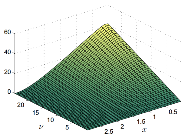
Source: Leung and Wang (2019) 

The optimal liquidation premium under the mean-reverting (exponential OU) model. The optimal liquidation premium tends to be large and may increase when the asset price is very low (i.e. for small x). This suggests that there is a high value from waiting to sell the asset later if the current price is low. As the asset price rises, the premium shrinks to zero, as expected. The investor finds no value in waiting any longer, resulting in an immediate sale. The optimal liquidation premium also varies with ν, which is the quantity of assets held. Source: Leung and Wang (2019) 

Reference 

T. Leung and Z. Wang, Optimal Risk Averse Timing of an Asset Sale: Trending vs Mean-Reverting Price Dynamics [pdf;link], Annals of Finance, Volume 15, Issue 1, pp.1–28, 2019.

Disclaimer: This post is not intended to be investment advice.