Python Correlation – A Practical Guide

The post “Python Correlation – A Practical Guide” first appeared on AlgoTrading101 Blog.

Excerpt

What is correlation?

A correlation is a relationship between two sets of data.

In the equity markets, for example, you may notice that stocks like Microsoft (MSFT) and Apple (AAPL) both tend to rise and fall at the same time. The price behavior between the two stocks is not an exact match, but there is enough similarity to say there is a relationship. In this scenario, we can say MSFT and AAPL have a positive correlation.

Further, there are often relationships across markets. For example, between equities and bonds, or precious metals. We often also see a correlation between financial instruments and economic data or even sentiment indicators.

Why do correlations matter?

There are several reasons why correlations are important, here a few benefits of tracking them in the markets –

1. Insights – keeping track of different relationships can provide insight into where the markets are headed. A good example is when the markets turned sharply lower in late February as a result of the Coronavirus escalation. The price of gold, which is known as an asset investors turn to when their mood for risky investments sours, rose sharply the trading day before the big initial drop in stocks. It acted as a warning signal for those equity traders mindful of the inverse correlation between the two.
2. Strength in correlated moves – It’s much easier to assess trends when there is a correlated move. In other words, if a bulk of the tech stocks on your watchlist are rising, it’s probably safe to say the sector is bullish, or that there is strong demand.
3. Diversification – To make sure you have some diversification in your portfolio, it’s a good idea to make sure the assets within it aren’t all strongly correlated to each other.
4. Signal confirmation – Let’s say you want to buy a stock because your analysis shows that it is bullish. You could analyze another stock with a positive correlation to make sure it provides a similar signal.

Correlation doesn’t imply causation

A popular saying among the statistics crowd is “correlation does not imply causation”. It comes up often and it’s important to understand its meaning.

Essentially, correlations can provide valuable insights but you’re bound to come across situations that might imply a correlation where a relationship does not exist.

As an example, data has shown a sharp rise in Netflix subscribers as a result of the lockdown that followed the Coronavirus escalation. The idea is that people are forced to stay at home and therefore are more likely to watch tv.

The same scenario has resulted in a rise in electricity bills. People are using more electricity at home compared to when they were at work all day.

If you were blindly comparing the rise in Netflix subscribers versus the rise in electricity usage during the month of lockdown, you might reasonably conclude that the two have a relationship.

However, having some perspective on the manner, it is clear that the two are not related and that it is not likely that fluctuations in one will impact the other moving forward. Rather, it is the lockdown, an external variable, that is the causation for both of these trends.

What is a correlation coefficient?

We’ve discussed that fluctuations in the stock prices of Apple and Microsoft tend to have a relationship. You might then notice other tech companies also correlate well with the two.

But not all relationships are equal and the correlation coefficient can help in assessing the strength of a correlation.

There are a few different ways of calculating a correlation coefficient but the most popular methods result in a number between -1 and +1.

The closer the number is to +1, the stronger the relationship. If the figure is close to -1, it indicates that there is a strong inverse relationship.

In the finance world, an inverse relationship is where one asset rises while the other drops. As one of the previous examples suggested, stocks and the price of gold have a long-standing inverse relationship.

The closer the correlation coefficient is to zero, the more likely it is that the two variables being compared don’t have any relationship to each other.

Breaking down the math to calculate the correlation coefficient

The above formula is what’s used to calculate a correlation coefficient using the Pearson method.

It might look a bit intimidating the first time you look at it (unless you’re a math pro ofcourse). But we will break down this formula and at the end of it you will see that it is just basic mathematics.

There are libraries available that can do this automatically, but the following example will show how we can make the calculation manually.

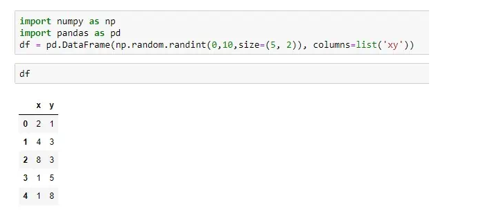
We will start by creating a dataset. We can use the Numpy library to create some random data for us. Here is the code:

import numpy as np
import pandas as pd
df = pd.DataFrame(np.random.randint(0,10,size=(5, 2)), columns=list('xy'))

The image below shows what my DataFrame looks like. If you’re following along, the data will look different for you as Numpy is filling in random numbers. But the format should look the same.

Now that we have a dataset, let’s move on to the formula. We will start by separating out the first part of the formula.

We can break this down further. Remember BODMAS? it states that we must perform what is in the brackets first.

For the formula above, we need to take each value of x and subtract it by the mean of x.

We can use the mean() function in Pandas to create the mean for us. Like this:

df.x.mean()

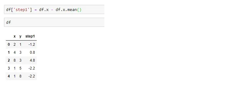
But we still need to subtract the mean from x. And we also need to temporarily store this information somewhere. Let’s create a new column for that and call it step1.

df['step1'] = df.x - df.x.mean()

This is what our DataFrame looks like at this point.

Now that we have the calculations needed for the first step. Let’s keep going.

The second step involves doing the same thing for the y column.

df['step2'] = df.y - df.y.mean()

That’s easy enough, what’s next?

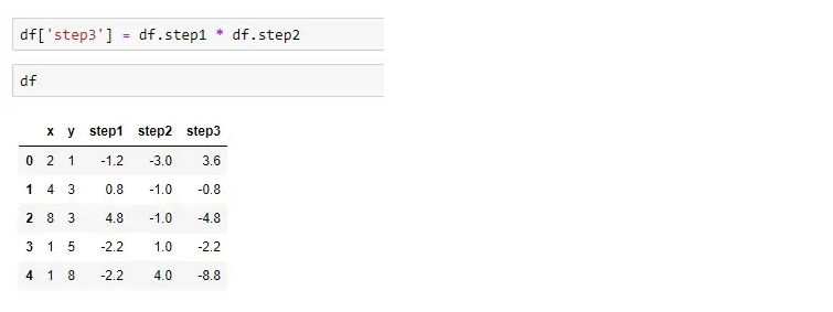
The formula is telling us that we need to take all the values we gathered in step 1 and multiply them by the values in step 2. We will store this in a new column labeled step3.

df['step3'] = df.step1 * df.step2

This is what the DataFrame looks like at this point:

We can now move on to the last operation in this part of the formula.

if you’re not familiar with this symbol:

It stands for sum. This means we need to add up all the values from the previous step.

step4 = df.step3.sum()

Great, we have summed up the values and have stored it in a variable called step4. We will come back to this later. For now, we can start on the second part of the formula.

Let’s follow the same steps and break down the formula.

Does this look familiar? we have already done this in step 1 so we can just use that data.

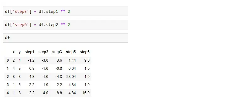
The next part of the formula tells us we have to square the results from step 1. We will store this data in a new column labeled step5.

df['step5'] = df.step1 ** 2

The next part of the formula tells us to do the same thing for the y values.

We can take the values that we created in step 2 and square them.

df['step6'] = df.step2 ** 2

This is what our DataFrame looks like at this point:

Let’s look at the next part of the formula:

This tells us that we have to take the sum of what we did in step 5 and multiply it with the sum of what we did in step 6.

step7 = df.step5.sum() * df.step6.sum()

Let’s keep going, almost there!

The last portion of this part is to simply take the square root of the figure from our previous step. We can use the Numpy library to calculate the square root.

step8 = np.sqrt(step7)

Now that we’ve done that, all that is left is to take the answer from the first part of the formula and divide it by the answer in the second part.

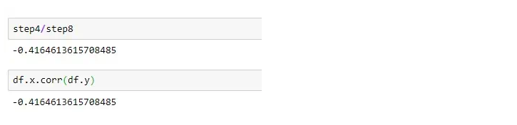
step4/step8

And there you have it, we’ve manually calculated a correlation coefficient. To make sure that the calculation is correct, we can will use the corr() function which is built into Pandas to calculate the coefficient.

df.x.corr(df.y)

Here is our final result. Your correlation coefficient will be different, but it should match the output from the Pandas calculation.

Visit AlgoTrading101 to read how to calculate the correlation coefficients for watchlist in Python.