This post shows how to apply the Particle Swarm Optimization (PSO) to estimate the Nelson-Siegel parameters using pso R package.

Particle Swarm Optimization (PSO)

PSO is a population-based optimization algorithm that mimics the collective behavior of birds or fish. It operates with a group of particles, each representing a possible solution to an optimization problem. These particles move through a solution space, continuously adjusting their positions and velocities. Each particle keeps track of its personal best solution and learns from the global best solution found by any particle in the population.

By balancing personal experience and global knowledge, PSO efficiently explores the solution space, gradually converging towards an optimal solution. The algorithm’s performance relies on relevant parameters like the number of particles, maximum velocity, and learning factors.

As with most topics, there is a wealth of extensive and valuable information about PSO available on Google, and this post does not duplicate it. Instead, I focus on applying the psoptim() function from the R package pso to solve practical problems.

R code

The following R code estimates the Nelson-Siegel parameters by using the PSO.

#========================================================#
# Quantitative Financial Econometrics & Derivatives 
# ML/DL using R, Python, Tensorflow by Sang-Heon Lee 
#
# https://shleeai.blogspot.com
#--------------------------------------------------------#
# Estimating the Nelson-Siegel model 
# using Particle Swarm Optimizer (PSO)
#========================================================#
 
graphics.off(); rm(list = ls())
library(pso) # psoptim
    
#-----------------------------------------------
# Objective function
#-----------------------------------------------
    objfunc <- function(para, y, m) {
        beta <- para[1:3]; la <- para[4]
        C  <- cbind(rep(1,length(m)),    
            (1-exp(-la*m))/(la*m),             
            (1-exp(-la*m))/(la*m)-exp(-la*m))
        return(sum((y - C%*%beta)^2))
    }
    
#=======================================================
# 1. Read data
#=======================================================
    
    # b1, b2, b3, lambda for comparisons
    ns_reg_para_rmse1 <- c(
        4.26219396, -4.08609206, -4.90893865,  
        0.02722607,  0.04883786)
    ns_reg_para_rmse2 <- c(
        4.97628654, -4.75365297, -6.40263059,  
        0.05046789,  0.04157326)
    
    str.zero <- "
        mat     rate1      rate2
        3       0.0781     0.0591
        6       0.1192     0.0931
        9       0.1579     0.1270
        12      0.1893     0.1654
        24      0.2669     0.3919
        36      0.3831     0.8192
        48      0.5489     1.3242
        60      0.7371     1.7623
        72      0.9523     2.1495
        84      1.1936     2.4994
        96      1.4275     2.7740
        108     1.6424     2.9798
        120     1.8326     3.1662
        144     2.1715     3.4829
        180     2.5489     3.7827
        240     2.8093     3.9696"
    
    df <- read.table(text = str.zero, header=TRUE)
    m  <- df$mat
    y1 <- df$rate1; y2 <- df$rate2
 
#==============================================================
# 2. Particle Swarm Optimizer 
#  : PSO Optimization with constraints
#==============================================================
    
    # NS estimation with 1st data
    y <- y1
    x_init <- c(y[16], y[1]-y[16], 
                2*y[6]-y[1]-y[16], 0.0609)
    
    set.seed(90)
    psopt<-psoptim(x_init, fn = objfunc,
                   lower = c(0, -20, -20, 0.015),
                   upper = c(20, 20,  20, 0.075),
                   y = y, m = m)
    
    nsptim_out1 <- c(psopt$par, sqrt(psopt$value/length(m)))
    
    # NS estimation with 2nd data
    y <- y2
    x_init <- c(y[16], y[1]-y[16], 
                2*y[6]-y[1]-y[16], 0.0609)
    
    set.seed(90)
    psopt <- psoptim(x_init, fn = objfunc, y = y, m = m,
         lower = c(0, -20, -20, 0.015),
         upper = c(20, 20,  20, 0.075),
         control = list(trace=1, REPORT=50,
             reltol=1e-4, abstol=1e-8,
             hybrid=TRUE, hybrid.control=list(maxit=10)))
    
    nsptim_out2 <- c(psopt$par, sqrt(psopt$value/length(m)))
    
#=======================================================
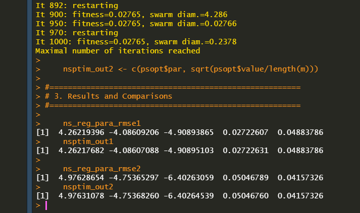
# 3. Results and Comparisons
#=======================================================
    
    ns_reg_para_rmse1
    nsptim_out1
    
    ns_reg_para_rmse2
    nsptim_out2
    

As can be seen in the following results, these simple examples yield the same outcomes with the given estimates.

Some research has applied hybrid particle swarm optimization and achieved promising results in financial applications such as asset allocation and yield curve fitting, among others, indicating the need for further exploration and investigation. Therefore, this post serves as a small step and starting point for guiding its usage. 

Originally posted on SHLee AI Financial Model blog.