Hierarchical Clustering in Python: A Comprehensive Implementation Guide – Part III

Author: Updated by Chainika Thakar (Originally written by Vibhu Singh)

Get started with an overview and key concepts of hierarchical clustering.

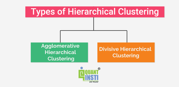
Types of hierarchical clustering

There are two types of hierarchical clustering:

• Agglomerative hierarchical clustering
• Divisive hierarchical clustering

Agglomerative Hierarchical Clustering

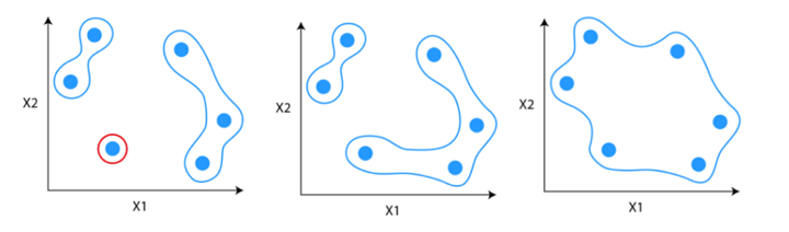
Agglomerative Hierarchical Clustering is the most common type of hierarchical clustering used to group objects in clusters based on their similarity. It’s a bottom-up approach where each observation starts in its own cluster, and pairs of clusters are merged as one moves up the hierarchy.

Let us find out a few important subpoints in this type of clustering as shown below.

How does Agglomerative Hierarchical Clustering work?

Suppose you have data points which you want to group in similar clusters.

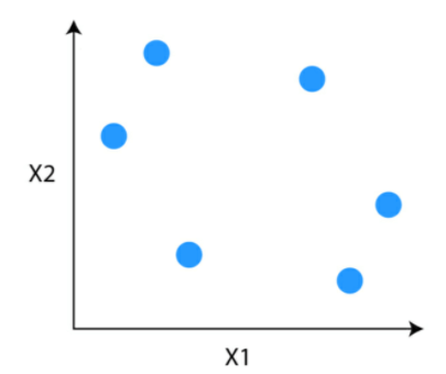
Step 1: The first step is to consider each data point to be a cluster.

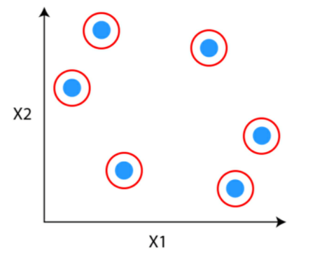
Step 2: Identify the two clusters that are similar and make them one cluster.

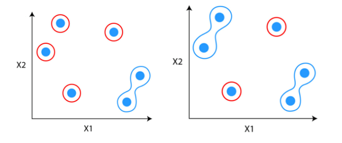
Step 3: Repeat the process until only single clusters remain

Divisive Hierarchical Clustering

Divisive hierarchical clustering is not used much in solving real-world problems. It works in the opposite way of agglomerative clustering. In this, we start with all the data points as a single cluster.

At each iteration, we separate the farthest points or clusters which are not similar until each data point is considered as an individual cluster. Here we are dividing the single clusters into n clusters, therefore the name divisive clustering.

Example of Divisive Hierarchical Clustering

In the context of trading, Divisive Hierarchical Clustering can be illustrated by starting with a cluster of all available stocks. As the algorithm progresses, it recursively divides this cluster into smaller subclusters based on dissimilarities in key financial indicators such as volatility, earnings growth, and price-to-earnings ratio. The process continues until individual stocks are isolated in distinct clusters, allowing traders to identify unique groups with similar financial characteristics for more targeted portfolio management.

---

How to do hierarchical clustering in Python?

To demonstrate the application of hierarchical clustering in Python, we will use the Iris dataset. The Iris dataset is one of the most common datasets that is used in machine learning for illustration purposes.

The Iris data has three types of Iris flowers which are three classes in the dependent variable. And it contains four independent variables which are sepal length, sepal width, petal length and petal width, all in cm. We will compare the original classes with the classes formed using hierarchical clustering methods.

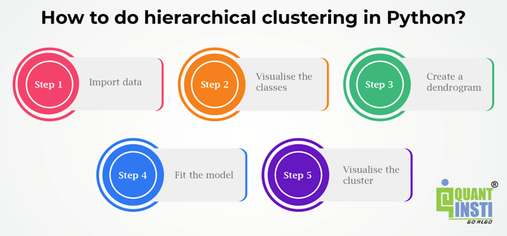
Let us take a look at the Python code with the steps below.

Step 1 – Import data

We will import the dataset from the sklearn library.

# Import libraries
import pandas as pd
import numpy as np
import matplotlib.pyplot as plt
from sklearn import datasets

# Import iris data 
iris = datasets.load_iris()

iris_data = pd.DataFrame(iris.data)
iris_data.columns = iris.feature_names
iris_data['flower_type'] = iris.target
iris_data.head()

Import_data.py hosted with ❤ by GitHub

Output:

	sepal length (cm)	sepal width (cm)	petal length (cm)	petal width (cm)	flower_type
0	5.1	3.5	1.4	0.2	0
1	4.9	3.0	1.4	0.2	0
2	4.7	3.2	1.3	0.2	0
3	4.6	3.1	1.5	0.2	0
4	5.0	3.6	1.4	0.2	0

Step 2 – Visualise the classes

iris_X = iris_data.iloc[:, [0, 1, 2,3]].values
iris_Y = iris_data.iloc[:,4].values

import matplotlib.pyplot as plt
plt.figure(figsize=(10, 7))
plt.scatter(iris_X[iris_Y == 0, 0], iris_X[iris_Y == 0, 1], s=100, c='blue', label='Type 1')
plt.scatter(iris_X[iris_Y == 1, 0], iris_X[iris_Y == 1, 1], s=100, c='yellow', label='Type 2')
plt.scatter(iris_X[iris_Y == 2, 0], iris_X[iris_Y == 2, 1], s=100, c='green', label='Type 3')
plt.legend()
plt.xlabel('Sample Index')
plt.ylabel('Euclidean Distance')
plt.show()

Visualise_Classes.py hosted with ❤ by GitHub

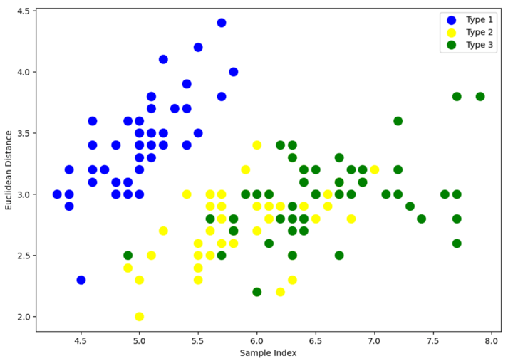
The above scatter plot shows that all three classes of Iris flowers overlap with each other. Our task is to form the cluster using hierarchical clustering and compare them with the original classes.

Step 3 – Create a dendrogram

We start by importing the library that will help to create dendrograms. The dendrogram helps to give a rough idea of the number of clusters.

import scipy.cluster.hierarchy as sc
# Plot dendrogram
plt.figure(figsize=(20, 7))
plt.title("Dendrograms")

# Create dendrogram
sc.dendrogram(sc.linkage(iris_X, method='ward'))

plt.title('Dendrogram')
plt.xlabel('Sample index')
plt.ylabel('Euclidean distance')

Create_dendrogram.py hosted with ❤ by GitHub

Output:

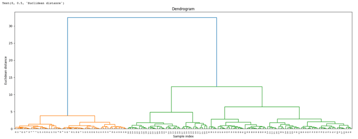
By looking at the above dendrogram, we divide the data into three clusters.

Step 4 – Fit the model

We instantiate Agglomerative Clustering. Pass Euclidean distance as the measure of the distance between points and ward linkage to calculate clusters’ proximity. Then we fit the model on our data points. Finally, we return an array of integers where the values correspond to the distinct categories using labels_ property.

from sklearn.cluster import AgglomerativeClustering

cluster = AgglomerativeClustering(
    n_clusters=3, affinity='euclidean', linkage='ward')

cluster.fit(iris_X)
labels = cluster.labels_
labels

Fit_model.py hosted with ❤ by GitHub

Output:

array([1, 1, 1, 1, 1, 1, 1, 1, 1, 1, 1, 1, 1, 1, 1, 1, 1, 1, 1, 1, 1, 1,
       1, 1, 1, 1, 1, 1, 1, 1, 1, 1, 1, 1, 1, 1, 1, 1, 1, 1, 1, 1, 1, 1,
       1, 1, 1, 1, 1, 1, 0, 0, 0, 0, 0, 0, 0, 0, 0, 0, 0, 0, 0, 0, 0, 0,
       0, 0, 0, 0, 0, 0, 0, 0, 0, 0, 0, 2, 0, 0, 0, 0, 0, 0, 0, 0, 0, 0,
       0, 0, 0, 0, 0, 0, 0, 0, 0, 0, 0, 0, 2, 0, 2, 2, 2, 2, 0, 2, 2, 2,
       2, 2, 2, 0, 0, 2, 2, 2, 2, 0, 2, 0, 2, 0, 2, 2, 0, 0, 2, 2, 2, 2,
       2, 0, 0, 2, 2, 2, 0, 2, 2, 2, 0, 2, 2, 2, 0, 2, 2, 0])

The above output shows the values of 0s, 1s, 2s, since we defined 4 clusters. 0 represents the points that belong to the first cluster and 1 represents points in the second cluster. Similarly, the third represents points in the third cluster.

Step 5 – Visualise the cluster

plt.figure(figsize=(10, 7))
plt.scatter(iris_X[labels == 0, 0], iris_X[labels == 0, 1], s = 100, c = 'blue', label = 'Type 1')
plt.scatter(iris_X[labels == 1, 0], iris_X[labels == 1, 1], s = 100, c = 'yellow', label = 'Type 2')
plt.scatter(iris_X[labels == 2, 0], iris_X[labels == 2, 1], s = 100, c = 'green', label = 'Type 3')
plt.legend()
plt.xlabel('Sample Index')
plt.ylabel('Euclidean Distance')
plt.show()

Visualise_cluster.py hosted with ❤ by GitHub

Output:

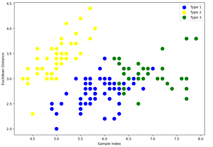
There is still an overlap between Type 1 and Type 3 clusters.

But if you compare with the original clusters in the Step 2 where we visualised the classes, the classification has improved quite a bit since the graph shows all three, i.e., Type 1, Type 2 and Type 3 not overlapping each other much.

Stay tuned to learn about hierarchical clustering in trading.

Originally posted on QuantInsti blog.